7.2 Change point models
The first example is a model of coal mining disasters in the U.K. for the years 1851–1962.16
Model with latent discrete parameter
Fonnesbeck et al. (2013, Section 3.1) provides a Poisson model of disaster \(D_t\) in year \(t\) with two rate parameters, an early rate (\(e\)) and late rate (\(l\)), that change at a given point in time \(s\). The full model expressed using a latent discrete parameter \(s\) is \[\begin{align*} e &\sim \textsf{exponential}(r_e) \\ l &\sim \textsf{exponential}(r_l) \\ s &\sim \textsf{uniform}(1, T) \\ D_t &\sim \textsf{Poisson}(t < s \; ? \; e \: : \: l) \end{align*}\]
The last line uses the conditional operator (also known as the ternary operator), which is borrowed from C and related languages. The conditional operator has the same behavior as its counterpart in C++.17
It uses a compact notation involving separating its three arguments by
a question mark (?) and a colon (:). The conditional
operator is defined by
\[
c \; ? \; x_1 \: : \: x_2
=
\begin{cases}
\ x_1 & \quad\text{if } c \text{ is true (i.e., non-zero), and} \\
\ x_2 & \quad\text{if } c \text{ is false (i.e., zero).}
\end{cases}
\]
Marginalizing out the discrete parameter
To code this model in Stan, the discrete parameter \(s\) must be marginalized out to produce a model defining the log of the probability function \(p(e,l,D_t)\). The full joint probability factors as \[\begin{align*} p(e,l,s,D) &= p(e) \, p(l) \, p(s) \, p(D \mid s, e, l) \\ &= \textsf{exponential}(e \mid r_e) \ \textsf{exponential}(l \mid r_l) \ \textsf{uniform}(s \mid 1, T) \\ &\qquad \prod_{t=1}^T \textsf{Poisson}(D_t \mid t < s \; ? \; e \: : \: l), \end{align*}\]
To marginalize, an alternative factorization into prior and likelihood is used, \[ p(e,l,D) = p(e,l) \, p(D \mid e,l), \] where the likelihood is defined by marginalizing \(s\) as \[\begin{align*} p(D \mid e,l) &= \sum_{s=1}^T p(s, D \mid e,l) \\ &= \sum_{s=1}^T p(s) \, p(D \mid s,e,l) \\ &= \sum_{s=1}^T \textsf{uniform}(s \mid 1,T) \, \prod_{t=1}^T \textsf{Poisson}(D_t \mid t < s \; ? \; e \: : \: l). \end{align*}\]
Stan operates on the log scale and thus requires the log likelihood, \[\begin{align*} \log p(D \mid e,l) &= \texttt{log}\mathtt{\_}\texttt{sum}\mathtt{\_}\texttt{exp}_{s=1}^T \left( \log \textsf{uniform}(s \mid 1, T) \vphantom{\sum_{t=1}^T}\right. \\ &\qquad \left. + \sum_{t=1}^T \log \textsf{Poisson}(D_t \mid t < s \; ? \; e \: : \: l) \right), \end{align*}\] where the log sum of exponents function is defined by \[ \texttt{log}\mathtt{\_}\texttt{sum}\mathtt{\_}\texttt{exp}_{n=1}^N \, \alpha_n = \log \sum_{n=1}^N \exp(\alpha_n). \]
The log sum of exponents function allows the model to be coded
directly in Stan using the built-in function log_sum_exp,
which provides both arithmetic stability and efficiency for mixture
model calculations.
Coding the model in Stan
The Stan program for the change point model is shown in
the figure below. The transformed parameter
lp[s] stores the quantity \(\log p(s, D \mid e, l)\).
data {
  real<lower=0> r_e;
  real<lower=0> r_l;

  int<lower=1> T;
  int<lower=0> D[T];
}
transformed data {
  real log_unif;
  log_unif = -log(T);
}
parameters {
  real<lower=0> e;
  real<lower=0> l;
}
transformed parameters {
  vector[T] lp;
  lp = rep_vector(log_unif, T);
  for (s in 1:T)
    for (t in 1:T)
      lp[s] = lp[s] + poisson_lpmf(D[t] | t < s ? e : l);
}
model {
  e ~ exponential(r_e);
  l ~ exponential(r_l);
  target += log_sum_exp(lp);
}
A change point model in which disaster rates D[t] have one rate,
e, before the change point and a different rate, l, after the
change point. The change point itself, s, is marginalized out as
described in the text.
Although the change-point model is coded directly, the doubly nested
loop used for s and t is quadratic in T. Luke Wiklendt pointed
out that a linear alternative can be achieved by the use of dynamic
programming similar to the forward-backward algorithm for Hidden
Markov models; he submitted a slight variant of the following code to
replace the transformed parameters block of the above Stan program.
transformed parameters {
    vector[T] lp;
    {
      vector[T + 1] lp_e;
      vector[T + 1] lp_l;
      lp_e[1] = 0;
      lp_l[1] = 0;
      for (t in 1:T) {
        lp_e[t + 1] = lp_e[t] + poisson_lpmf(D[t] | e);
        lp_l[t + 1] = lp_l[t] + poisson_lpmf(D[t] | l);
      }
      lp = rep_vector(log_unif + lp_l[T + 1], T)
           + head(lp_e, T) - head(lp_l, T);
    }
  }
As should be obvious from looking at it, it has linear complexity in
T rather than quadratic. The result for the mining-disaster
data is about 20 times faster; the improvement will be greater for
larger T.
The key to understanding Wiklendt’s dynamic programming version is to
see that head(lp_e) holds the forward values, whereas
lp_l[T + 1] - head(lp_l, T) holds the backward values; the
clever use of subtraction allows lp_l to be accumulated
naturally in the forward direction.
Fitting the model with MCMC
This model is easy to fit using MCMC with NUTS in its default configuration. Convergence is fast and sampling produces roughly one effective sample every two iterations. Because it is a relatively small model (the inner double loop over time is roughly 20,000 steps), it is fast.
The value of lp for each iteration for each change point is
available because it is declared as a transformed parameter. If the
value of lp were not of interest, it could be coded as a local
variable in the model block and thus avoid the I/O overhead of saving
values every iteration.
Posterior distribution of the discrete change point
The value of lp[s] in a given iteration is given by \(\log p(s,D \mid e,l)\) for the values of the early and late rates, \(e\) and \(l\),
in the iteration. In each iteration after convergence, the early and
late disaster rates, \(e\) and \(l\), are drawn from the posterior
\(p(e,l \mid D)\) by MCMC sampling and the associated lp calculated.
The value of lp may be normalized to calculate \(p(s \mid e,l,D)\) in
each iteration, based on on the current values of \(e\) and \(l\).
Averaging over iterations provides an unnormalized probability
estimate of the change point being \(s\) (see below for the normalizing
constant),
\[\begin{align*}
p(s \mid D) &\propto q(s \mid D) \\
&= \frac{1}{M} \sum_{m=1}^{M} \exp(\texttt{lp}[m,s]).
\end{align*}\]
where \(\texttt{lp}[m,s]\) represents the value of lp in
posterior draw \(m\) for change point \(s\). By averaging over draws,
\(e\) and \(l\) are themselves marginalized out, and the result has no
dependence on a given iteration’s value for \(e\) and \(l\). A final
normalization then produces the quantity of interest, the posterior
probability of the change point being \(s\) conditioned on the data \(D\),
\[
p(s \mid D) = \frac{q(s \mid D)}{\sum_{s'=1}^T q(s' \mid D)}.
\]
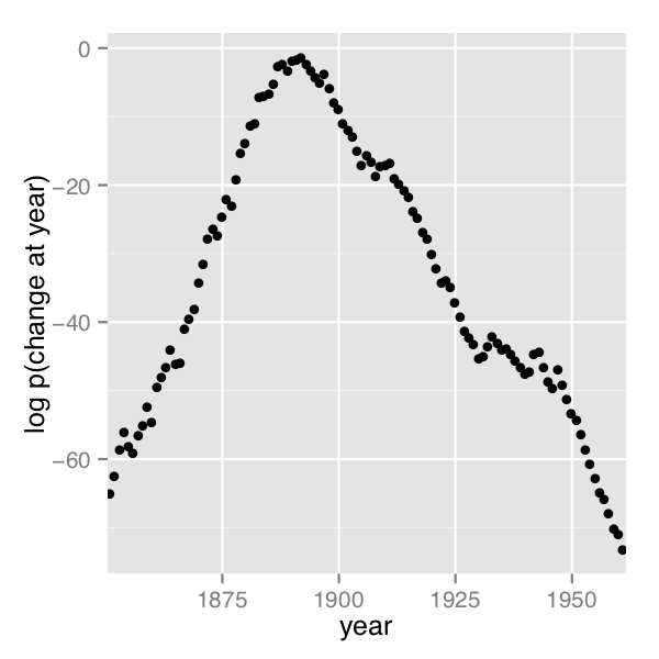
A plot of the values of \(\log p(s \mid D)\) computed using Stan 2.4’s default MCMC implementation is shown in the posterior plot.
Log probability of change point being in year, calculated analytically.

Figure 7.1: Analytical change-point posterior
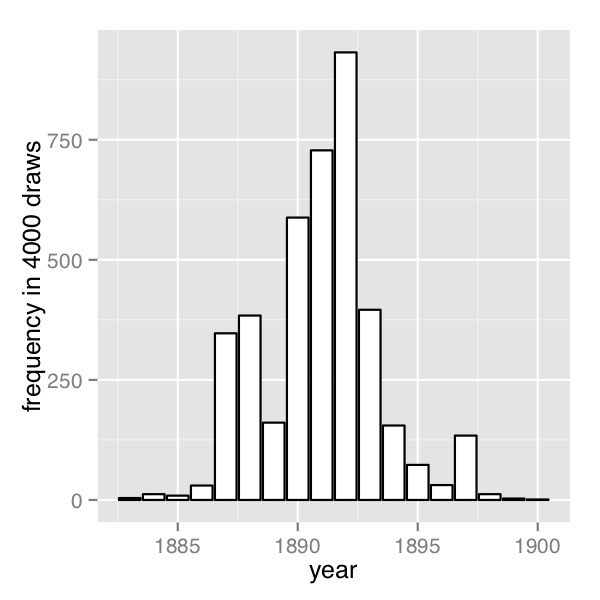
The frequency of change points generated by sampling the discrete change points.

Figure 7.2: Sampled change-point posterior
In order their range of estimates be visible, the first plot is on the log scale and the second plot on the linear scale; note the narrower range of years in the second plot resulting from sampling. The posterior mean of \(s\) is roughly 1891.
Discrete sampling
The generated quantities block may be used to draw discrete parameter
values using the built-in pseudo-random number generators. For
example, with lp defined as above, the following program
draws a random value for s at every iteration.
generated quantities {
  int<lower=1,upper=T> s;
  s = categorical_logit_rng(lp);
}
A posterior histogram of draws for \(s\) is shown on the second change point posterior figure above.
Compared to working in terms of expectations, discrete sampling is
highly inefficient, especially for tails of distributions, so this
approach should only be used if draws from a distribution are
explicitly required. Otherwise, expectations should be computed in
the generated quantities block based on the posterior distribution for
s given by softmax(lp).
Posterior covariance
The discrete sample generated for \(s\) can be used to calculate
covariance with other parameters. Although the sampling approach is
straightforward, it is more statistically efficient (in the sense of
requiring far fewer iterations for the same degree of accuracy) to
calculate these covariances in expectation using lp.
Multiple change points
There is no obstacle in principle to allowing multiple change points.
The only issue is that computation increases from linear to quadratic
in marginalizing out two change points, cubic for three change points,
and so on. There are three parameters, e, m, and
l, and two loops for the change point and then one over time,
with log densities being stored in a matrix.
matrix[T, T] lp;
lp = rep_matrix(log_unif, T);
for (s1 in 1:T)
  for (s2 in 1:T)
    for (t in 1:T)
      lp[s1,s2] = lp[s1,s2]
        + poisson_lpmf(D[t] | t < s1 ? e : (t < s2 ? m : l));
The matrix can then be converted back to a vector using
to_vector before being passed to log_sum_exp.
References
Fonnesbeck, Chris, Anand Patil, David Huard, and John Salvatier. 2013. PyMC User’s Guide.