15.2 HMC Algorithm Parameters
The Hamiltonian Monte Carlo algorithm has three parameters which must be set,
- discretization time \(\epsilon\),
- metric \(M\), and
- number of steps taken \(L\).
In practice, sampling efficiency, both in terms of iteration speed and iterations per effective sample, is highly sensitive to these three tuning parameters Neal (2011), Hoffman and Gelman (2014).
If \(\epsilon\) is too large, the leapfrog integrator will be inaccurate and too many proposals will be rejected. If \(\epsilon\) is too small, too many small steps will be taken by the leapfrog integrator leading to long simulation times per interval. Thus the goal is to balance the acceptance rate between these extremes.
If \(L\) is too small, the trajectory traced out in each iteration will be too short and sampling will devolve to a random walk. If \(L\) is too large, the algorithm will do too much work on each iteration.
If the inverse metric \(M^{-1}\) is a poor estimate of the posterior covariance, the step size \(\epsilon\) must be kept small to maintain arithmetic precision. This would lead to a large \(L\) to compensate.
Integration Time
The actual integration time is \(L \, \epsilon\), a function of number of steps. Some interfaces to Stan set an approximate integration time \(t\) and the discretization interval (step size) \(\epsilon\). In these cases, the number of steps will be rounded down as
\[ L = \left\lfloor \frac{t}{\epsilon} \right\rfloor. \]
and the actual integration time will still be \(L \, \epsilon\).
Automatic Parameter Tuning
Stan is able to automatically optimize \(\epsilon\) to match an acceptance-rate target, able to estimate \(M\) based on warmup sample iterations, and able to dynamically adapt \(L\) on the fly during sampling (and during warmup) using the no-U-turn sampling (NUTS) algorithm Hoffman and Gelman (2014).
Warmup Epochs Figure. Adaptation during warmup occurs in three stages: an initial fast adaptation interval (I), a series of expanding slow adaptation intervals (II), and a final fast adaptation interval (III). For HMC, both the fast and slow intervals are used for adapting the step size, while the slow intervals are used for learning the (co)variance necessitated by the metric. Iteration numbering starts at 1 on the left side of the figure and increases to the right.
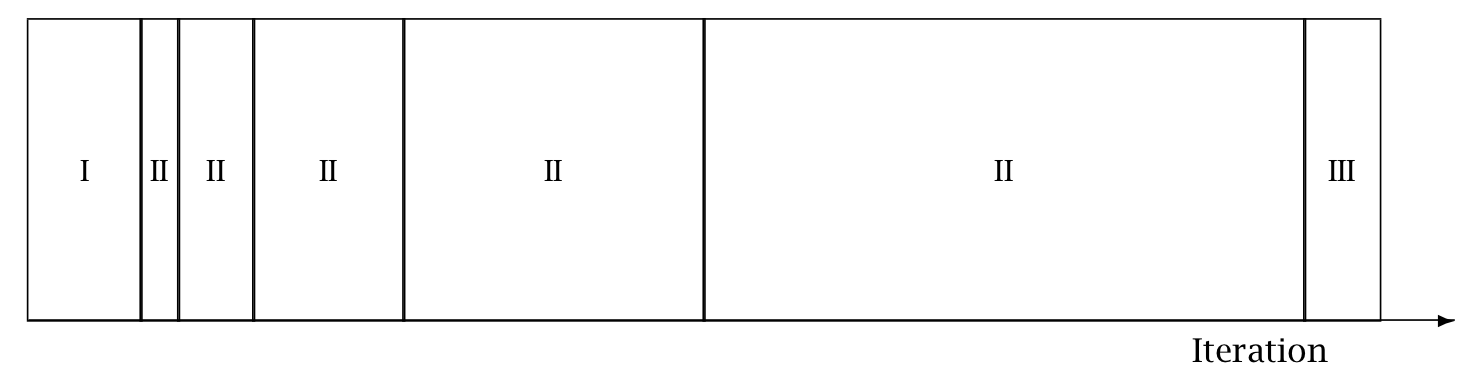
When adaptation is engaged (it may be turned off by fixing a step size and metric), the warmup period is split into three stages, as illustrated in the warmup adaptation figure, with two fast intervals surrounding a series of growing slow intervals. Here fast and slow refer to parameters that adapt using local and global information, respectively; the Hamiltonian Monte Carlo samplers, for example, define the step size as a fast parameter and the (co)variance as a slow parameter. The size of the the initial and final fast intervals and the initial size of the slow interval are all customizable, although user-specified values may be modified slightly in order to ensure alignment with the warmup period.
The motivation behind this partitioning of the warmup period is to allow for more robust adaptation. The stages are as follows.
In the initial fast interval the chain is allowed to converge towards the typical set,20 with only parameters that can learn from local information adapted.
After this initial stage parameters that require global information, for example (co)variances, are estimated in a series of expanding, memoryless windows; often fast parameters will be adapted here as well.
Lastly, the fast parameters are allowed to adapt to the final update of the slow parameters.
These intervals may be controlled through the following configuration parameters, all of which must be positive integers:
Adaptation Parameters Table. The parameters controlling adaptation and their default values.
| parameter | description | default |
|---|---|---|
| initial buffer | width of initial fast adaptation interval | 75 |
| term buffer | width of final fast adaptation interval | 50 |
| window | initial width of slow adaptation interval | 25 |
Discretization-Interval Adaptation Parameters
Stan’s HMC algorithms utilize dual averaging Nesterov (2009) to optimize the step size.21
This warmup optimization procedure is extremely flexible and for completeness, Stan exposes each tuning option for dual averaging, using the notation of Hoffman and Gelman (2014). In practice, the efficacy of the optimization is sensitive to the value of these parameters, but we do not recommend changing the defaults without experience with the dual-averaging algorithm. For more information, see the discussion of dual averaging in Hoffman-Gelman:2014.
The full set of dual-averaging parameters are
Step Size Adaptation Parameters Table The parameters controlling step size adaptation, with constraints and default values.
| parameter | description | constraint | default |
|---|---|---|---|
delta |
target Metropolis acceptance rate | [0, 1] | 0.8 |
gamma |
adaptation regularization scale | (0, infty) | 0.05 |
kappa |
adaptation relaxation exponent | (0, infty) | 0.75 |
t_0 |
adaptation iteration offset | (0, infty) | 10 |
By setting the target acceptance parameter \(\delta\) to a value closer to 1 (its value must be strictly less than 1 and its default value is 0.8), adaptation will be forced to use smaller step sizes. This can improve sampling efficiency (effective sample size per iteration) at the cost of increased iteration times. Raising the value of \(\delta\) will also allow some models that would otherwise get stuck to overcome their blockages.
Step-Size Jitter
All implementations of HMC use numerical integrators requiring a step size (equivalently, discretization time interval). Stan allows the step size to be adapted or set explicitly. Stan also allows the step size to be “jittered” randomly during sampling to avoid any poor interactions with a fixed step size and regions of high curvature. The jitter is a proportion that may be added or subtracted, so the maximum amount of jitter is 1, which will cause step sizes to be selected in the range of 0 to twice the adapted step size. The default value is 0, producing no jitter.
Small step sizes can get HMC samplers unstuck that would otherwise get stuck with higher step sizes. The downside is that jittering below the adapted value will increase the number of leapfrog steps required and thus slow down iterations, whereas jittering above the adapted value can cause premature rejection due to simulation error in the Hamiltonian dynamics calculation. See Neal (2011) for further discussion of step-size jittering.
Euclidean Metric
All HMC implementations in Stan utilize quadratic kinetic energy functions which are specified up to the choice of a symmetric, positive-definite matrix known as a mass matrix or, more formally, a metric Betancourt (2017).
If the metric is constant then the resulting implementation is known as Euclidean HMC. Stan allows a choice among three Euclidean HMC implementations,
- a unit metric (diagonal matrix of ones),
- a diagonal metric (diagonal matrix with positive diagonal entries), and
- a dense metric (a dense, symmetric positive definite matrix)
to be configured by the user.
If the metric is specified to be diagonal, then regularized variances are estimated based on the iterations in each slow-stage block (labeled II in the warmup adaptation stages figure). Each of these estimates is based only on the iterations in that block. This allows early estimates to be used to help guide warmup and then be forgotten later so that they do not influence the final covariance estimate.
If the metric is specified to be dense, then regularized covariance estimates will be carried out, regularizing the estimate to a diagonal matrix, which is itself regularized toward a unit matrix.
Variances or covariances are estimated using Welford accumulators to avoid a loss of precision over many floating point operations.
Warmup Times and Estimating the Metric
The metric can compensate for linear (i.e. global) correlations in the posterior which can dramatically improve the performance of HMC in some problems. This requires knowing the global correlations.
In complex models, the global correlations are usually difficult, if not impossible, to derive analytically; for example, nonlinear model components convolve the scales of the data, so standardizing the data does not always help. Therefore, Stan estimates these correlations online with an adaptive warmup. In models with strong nonlinear (i.e. local) correlations this learning can be slow, even with regularization. This is ultimately why warmup in Stan often needs to be so long, and why a sufficiently long warmup can yield such substantial performance improvements.
Nonlinearity
The metric compensates for only linear (equivalently global or position-independent) correlations in the posterior. The hierarchical parameterizations, on the other hand, affect some of the nasty nonlinear (equivalently local or position-dependent) correlations common in hierarchical models.22
One of the biggest difficulties with dense metrics is the estimation of the metric itself which introduces a bit of a chicken-and-egg scenario; in order to estimate an appropriate metric for sampling, convergence is required, and in order to converge, an appropriate metric is required.
Dense vs. Diagonal Metrics
Statistical models for which sampling is problematic are not typically dominated by linear correlations for which a dense metric can adjust. Rather, they are governed by more complex nonlinear correlations that are best tackled with better parameterizations or more advanced algorithms, such as Riemannian HMC.
Warmup Times and Curvature
MCMC convergence time is roughly equivalent to the autocorrelation time. Because HMC (and NUTS) chains tend to be lowly autocorrelated they also tend to converge quite rapidly.
This only applies when there is uniformity of curvature across the posterior, an assumption which is violated in many complex models. Quite often, the tails have large curvature while the bulk of the posterior mass is relatively well-behaved; in other words, warmup is slow not because the actual convergence time is slow but rather because the cost of an HMC iteration is more expensive out in the tails.
Poor behavior in the tails is the kind of pathology that can be uncovered by running only a few warmup iterations. By looking at the acceptance probabilities and step sizes of the first few iterations provides an idea of how bad the problem is and whether it must be addressed with modeling efforts such as tighter priors or reparameterizations.
NUTS and its Configuration
The no-U-turn sampler (NUTS) automatically selects an appropriate number of leapfrog steps in each iteration in order to allow the proposals to traverse the posterior without doing unnecessary work. The motivation is to maximize the expected squared jump distance (see, e.g., Roberts, Gelman, and Gilks (1997)) at each step and avoid the random-walk behavior that arises in random-walk Metropolis or Gibbs samplers when there is correlation in the posterior. For a precise definition of the NUTS algorithm and a proof of detailed balance, see Hoffman and Gelman (2014).
NUTS generates a proposal by starting at an initial position determined by the parameters drawn in the last iteration. It then generates an independent standard normal random momentum vector. It then evolves the initial system both forwards and backwards in time to form a balanced binary tree. At each iteration of the NUTS algorithm the tree depth is increased by one, doubling the number of leapfrog steps and effectively doubles the computation time. The algorithm terminates in one of two ways, either
- the NUTS criterion (i.e., a U-turn in Euclidean space on a subtree) is satisfied for a new subtree or the completed tree, or
- the depth of the completed tree hits the maximum depth allowed.
Rather than using a standard Metropolis step, the final parameter value is selected via multinomial sampling with a bias toward the second half of the steps in the trajectory Betancourt (2016b).23
Configuring the no-U-turn sample involves putting a cap on the depth of the trees that it evaluates during each iteration. This is controlled through a maximum depth parameter. The number of leapfrog steps taken is then bounded by 2 to the power of the maximum depth minus 1.
Both the tree depth and the actual number of leapfrog steps computed are reported along with the parameters in the output as treedepth__ and n_leapfrog__, respectively. Because the final subtree may only be partially constructed, these two will always satisfy
\[ 2^{\mathrm{treedepth} - 1} - 1 \ < \ N_{\mathrm{leapfrog}} \ \le \ 2^{\mathrm{treedepth} } - 1. \]
Tree depth is an important diagnostic tool for NUTS. For example, a tree depth of zero occurs when the first leapfrog step is immediately rejected and the initial state returned, indicating extreme curvature and poorly-chosen step size (at least relative to the current position). On the other hand, a tree depth equal to the maximum depth indicates that NUTS is taking many leapfrog steps and being terminated prematurely to avoid excessively long execution time. Taking very many steps may be a sign of poor adaptation, may be due to targeting a very high acceptance rate, or may simply indicate a difficult posterior from which to sample. In the latter case, reparameterization may help with efficiency. But in the rare cases where the model is correctly specified and a large number of steps is necessary, the maximum depth should be increased to ensure that that the NUTS tree can grow as large as necessary.
References
Neal, Radford. 2011. “MCMC Using Hamiltonian Dynamics.” In Handbook of Markov Chain Monte Carlo, edited by Steve Brooks, Andrew Gelman, Galin L. Jones, and Xiao-Li Meng, 116–62. Chapman; Hall/CRC.
Hoffman, Matthew D., and Andrew Gelman. 2014. “The No-U-Turn Sampler: Adaptively Setting Path Lengths in Hamiltonian Monte Carlo.” Journal of Machine Learning Research 15: 1593–1623. http://jmlr.org/papers/v15/hoffman14a.html.
Nesterov, Y. 2009. “Primal-Dual Subgradient Methods for Convex Problems.” Mathematical Programming 120 (1). Springer: 221–59.
Betancourt, Michael. 2017. “A Conceptual Introduction to Hamiltonian Monte Carlo.” arXiv 1701.02434. https://arxiv.org/abs/1701.02434.
Roberts, G.O., Andrew Gelman, and Walter R. Gilks. 1997. “Weak Convergence and Optimal Scaling of Random Walk Metropolis Algorithms.” Annals of Applied Probability 7 (1): 110–20.
Betancourt, Michael. 2016b. “Identifying the Optimal Integration Time in Hamiltonian Monte Carlo.” arXiv 1601.00225. https://arxiv.org/abs/1601.00225.
The typical set is a concept borrowed from information theory and refers to the neighborhood (or neighborhoods in multimodal models) of substantial posterior probability mass through which the Markov chain will travel in equilibrium.↩
This optimization of step size during adaptation of the sampler should not be confused with running Stan’s optimization method.↩
In Riemannian HMC the metric compensates for nonlinear correlations.↩
Stan previously used slice sampling along the trajectory, following the original NUTS paper of Hoffman and Gelman (2014).↩