26.2 Plotting multiples
A standard posterior predictive check would plot a histogram of each replicated data set along with the original data set and compare them by eye. For this purpose, only a few replications are needed. These should be taken by thinning a larger set of replications down to the size needed to ensure rough independence of the replications.
Here’s a complete example where the model is a simple Poisson with a weakly informative exponential prior with a mean of 10 and standard deviation of 10.
data {
  int<lower = 0> N;
  int<lower = 0> y[N];
}
transformed data {
  real<lower = 0> mean_y = mean(to_vector(y));
  real<lower = 0> sd_y = sd(to_vector(y));
}
parameters {
  real<lower = 0> lambda;
}
model {
  y ~ poisson(lambda);
  lambda ~ exponential(0.2);
}
generated quantities {
  int<lower = 0> y_rep[N] = poisson_rng(rep_array(lambda, N));
  real<lower = 0> mean_y_rep = mean(to_vector(y_rep));
  real<lower = 0> sd_y_rep = sd(to_vector(y_rep));
  int<lower = 0, upper = 1> mean_gte = (mean_y_rep >= mean_y);
  int<lower = 0, upper = 1> sd_gte = (sd_y_rep >= sd_y);
}
The generated quantities block creates a variable y_rep for the
replicated data, variables mean_y_rep and sd_y_rep for the
statistics of the replicated data, and indicator variables
mean_gte and sd_gte for whether the replicated statistic
is greater than or equal to the statistic applied to the original
data.
Now consider generating data \(y \sim \textrm{Poisson}(5)\). The resulting small multiples plot shows the original data plotted in the upper left and eight different posterior replications plotted in the remaining boxes.
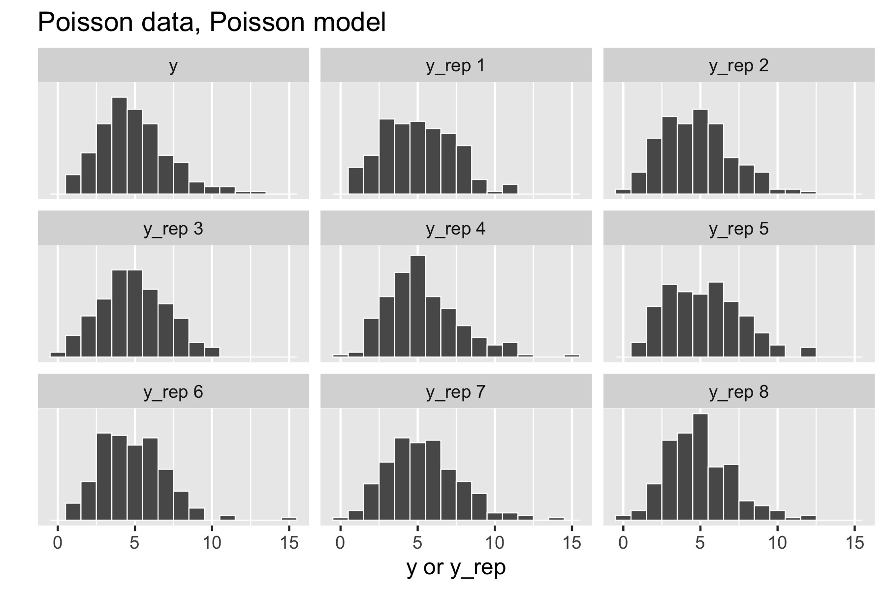
Figure 26.1: Posterior predictive checks for Poisson data generating process and Poisson model.
With a Poisson data-generating process and Poisson model, the posterior replications look similar to the original data. If it were easy to pick the original data out of the lineup, there would be a problem.
Now consider generating over-dispersed data \(y \sim \textrm{negative-binomial2}(5, 1).\) This has the same mean as \(\textrm{Poisson}(5)\), namely \(5\), but a standard deviation of \(\sqrt{5 + 5^2 /1} \approx 5.5.\) There is no way to fit this data with the Poisson model, because a variable distributed as \(\textrm{Poisson}(\lambda)\) has mean \(\lambda\) and standard deviation \(\sqrt{\lambda},\) which is \(\sqrt{5}\) for \(\textrm{Poisson}(5).\) Here’s the resulting small multiples plot, again with original data in the upper left.
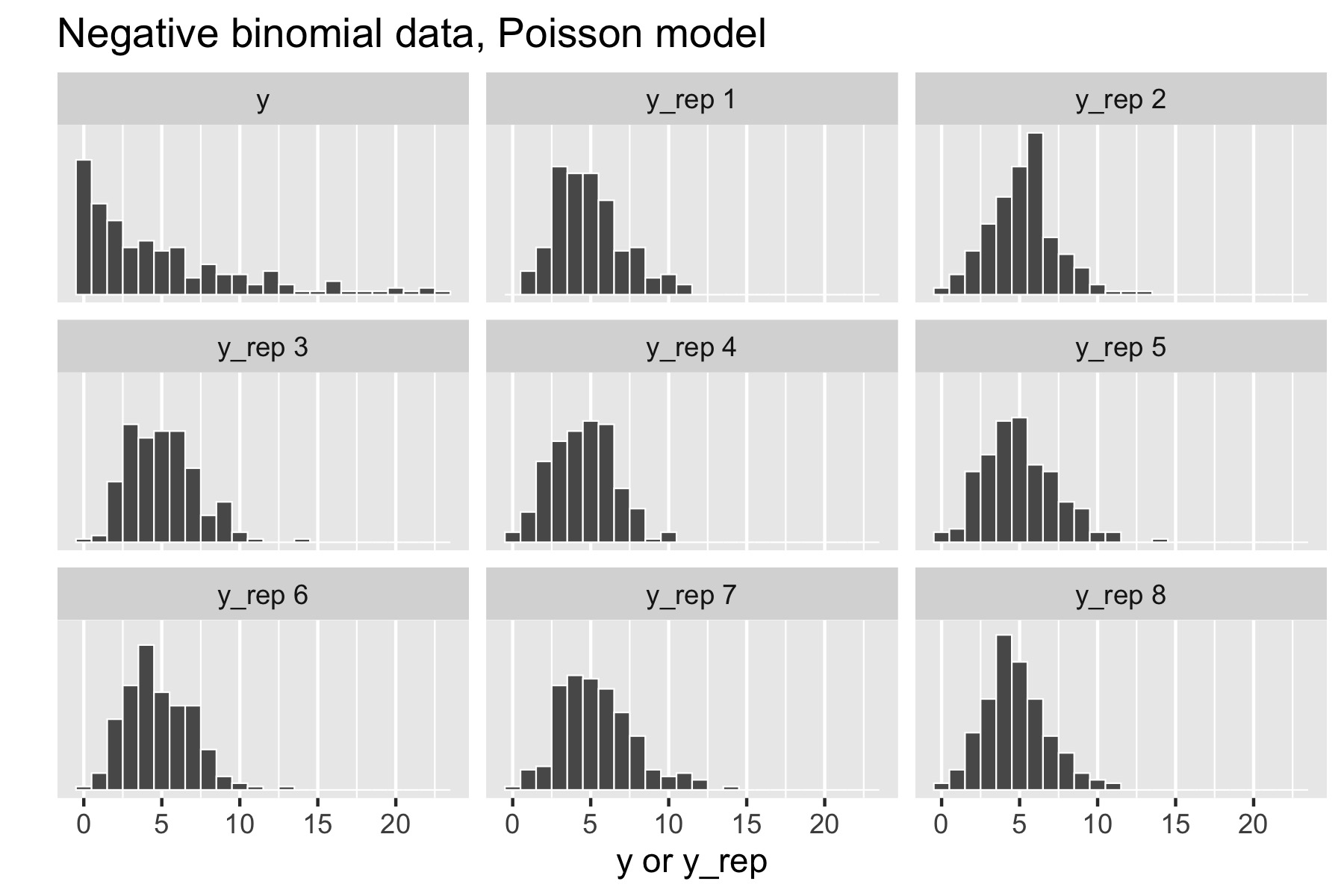
Figure 26.2: Posterior predictive checks for negative binomial data generating process and Poisson model.
This time, the original data stands out in stark contrast to the replicated data sets, all of which are clearly more symmetric and lower variance than the original data. That is, the model’s not appropriately capturing the variance of the data.