Posterior and Prior Predictive Checks

Posterior predictive checks are a way of measuring whether a model does a good job of capturing relevant aspects of the data, such as means, standard deviations, and quantiles (Rubin 1984; Andrew Gelman, Meng, and Stern 1996). Posterior predictive checking works by simulating new replicated data sets based on the fitted model parameters and then comparing statistics applied to the replicated data set with the same statistic applied to the original data set.

Prior predictive checks evaluate the prior the same way. Specifically, they evaluate what data sets would be consistent with the prior. They will not be calibrated with actual data, but extreme values help diagnose priors that are either too strong, too weak, poorly shaped, or poorly located.

Prior and posterior predictive checks are two cases of the general concept of predictive checks, just conditioning on different things (no data and the observed data, respectively). For hierarchical models, there are intermediate versions, as discussed in the section on hierarchical models and mixed replication.

Simulating from the posterior predictive distribution

The posterior predictive distribution is the distribution over new observations given previous observations. It’s predictive in the sense that it’s predicting behavior on new data that is not part of the training set. It’s posterior in that everything is conditioned on observed data $y$.

The posterior predictive distribution for replications $y^{\text{rep}}$ of the original data set $y$ given model parameters $\theta$ is defined by $$p(y^{\text{rep}}\mid y)=\int p(y^{\text{rep}}\mid \theta )\cdot p(\theta \mid y)\text{d}\theta .$$

As with other posterior predictive quantities, generating a replicated data set $y^{\text{rep}}$ from the posterior predictive distribution is straightforward using the generated quantities block. Consider a simple regression model with parameters $\theta =(\alpha ,\beta ,\sigma ).$

data {
  int<lower=0> N;
  vector[N] x;
  vector[N] y;
}
parameters {
  real alpha;
  real beta;
  real<lower=0> sigma;
}
model {
  alpha ~ normal(0, 2);
  beta ~ normal(0, 1);
  sigma ~ normal(0, 1);
  y ~ normal(alpha + beta * x, sigma);
}

To generate a replicated data set y_rep for this simple model, the following generated quantities block suffices.

generated quantities {
  array[N] real y_rep = normal_rng(alpha + beta * x, sigma);
}

The vectorized form of the normal random number generator is used with the original predictors x and the model parameters alpha, beta, and sigma. The replicated data variable y_rep is declared to be the same size as the original data y, but instead of a vector type, it is declared to be an array of reals to match the return type of the function normal_rng. Because the vector and real array types have the same dimensions and layout, they can be plotted against one another and otherwise compared during downstream processing.

The posterior predictive sampling for posterior predictive checks is different from usual posterior predictive sampling discussed in the chapter on posterior predictions in that the original predictors $x$ are used. That is, the posterior predictions are for the original data.

Plotting multiples

A standard posterior predictive check would plot a histogram of each replicated data set along with the original data set and compare them by eye. For this purpose, only a few replications are needed. These should be taken by thinning a larger set of replications down to the size needed to ensure rough independence of the replications.

Here’s a complete example where the model is a simple Poisson with a weakly informative exponential prior with a mean of 10 and standard deviation of 10.

data {
  int<lower=0> N;
  array[N] int<lower=0> y;
}
transformed data {
  real<lower=0> mean_y = mean(to_vector(y));
  real<lower=0> sd_y = sd(to_vector(y));
}
parameters {
  real<lower=0> lambda;
}
model {
  y ~ poisson(lambda);
  lambda ~ exponential(0.2);
}
generated quantities {
  array[N] int<lower=0> y_rep = poisson_rng(rep_array(lambda, N));
  real<lower=0> mean_y_rep = mean(to_vector(y_rep));
  real<lower=0> sd_y_rep = sd(to_vector(y_rep));
  int<lower=0, upper=1> mean_gte = (mean_y_rep >= mean_y);
  int<lower=0, upper=1> sd_gte = (sd_y_rep >= sd_y);
}

The generated quantities block creates a variable y_rep for the replicated data, variables mean_y_rep and sd_y_rep for the statistics of the replicated data, and indicator variables mean_gte and sd_gte for whether the replicated statistic is greater than or equal to the statistic applied to the original data.

Now consider generating data $y\sim \text{Poisson}(5)$. The resulting small multiples plot shows the original data plotted in the upper left and eight different posterior replications plotted in the remaining boxes.

Posterior predictive checks for Poisson data generating process and Poisson model.

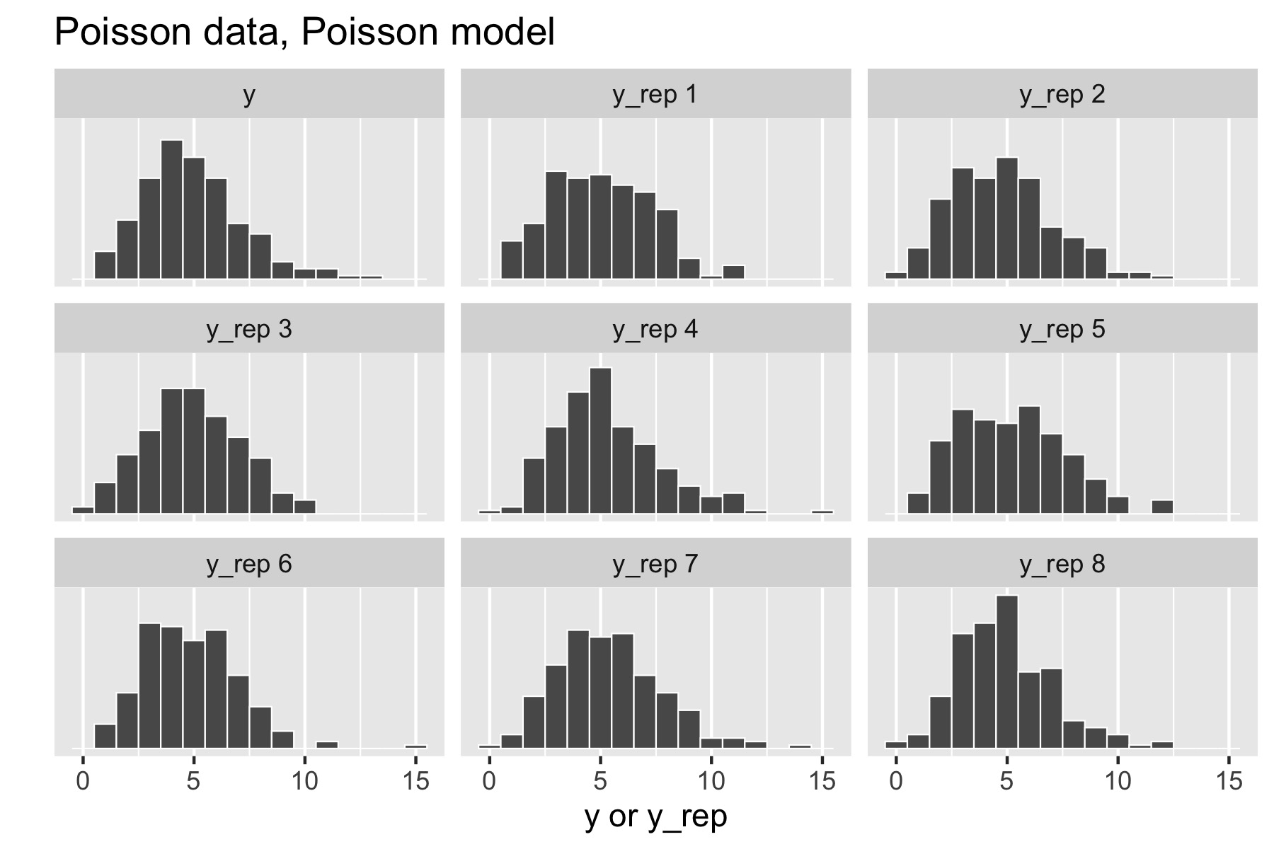
With a Poisson data-generating process and Poisson model, the posterior replications look similar to the original data. If it were easy to pick the original data out of the lineup, there would be a problem.

Now consider generating over-dispersed data $y\sim \text{negative-binomial2}(5,1).$ This has the same mean as $\text{Poisson}(5)$, namely $5$, but a standard deviation of $\sqrt{5+5^2/1}\approx 5.5.$ There is no way to fit this data with the Poisson model, because a variable distributed as $\text{Poisson}(\lambda )$ has mean $\lambda$ and standard deviation $\sqrt{\lambda },$ which is $\sqrt{5}$ for $\text{Poisson}(5).$ Here’s the resulting small multiples plot, again with original data in the upper left.

Posterior predictive checks for negative binomial data generating process and Poisson model.

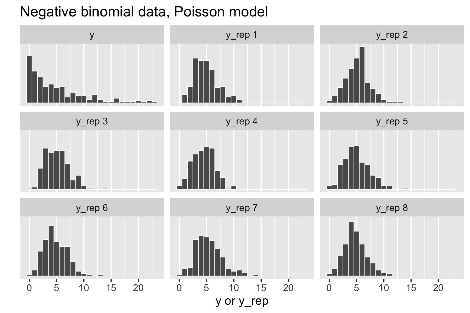
This time, the original data stands out in stark contrast to the replicated data sets, all of which are clearly more symmetric and lower variance than the original data. That is, the model’s not appropriately capturing the variance of the data.

Posterior ‘’p-values’’

If a model captures the data well, summary statistics such as sample mean and standard deviation, should have similar values in the original and replicated data sets. This can be tested by means of a p-value-like statistic, which here is just the probability the test statistic $s(\cdot )$ in a replicated data set exceeds that in the original data, $$Pr[s(y^{\text{rep}})\ge s(y)\mid y]=\int \text{I}(s(y^{\text{rep}})\ge s(y)\mid y)\cdot p(y^{\text{rep}}\mid y)\text{d}{y}^{\text{rep}}.$$ It is important to note that ‘’p-values’’ is in quotes because these statistics are not classically calibrated, and thus will not in general have a uniform distribution even when the model is well specified (Bayarri and Berger 2000).

Nevertheless, values of this statistic very close to zero or one are cause for concern that the model is not fitting the data well. Unlike a visual test, this p-value-like test is easily automated for bulk model fitting.

To calculate event probabilities in Stan, it suffices to define indicator variables that take on value 1 if the event occurs and 0 if it does not. The posterior mean is then the event probability. For efficiency, indicator variables are defined in the generated quantities block.

generated quantities {
  int<lower=0, upper=1> mean_gt;
  int<lower=0, upper=1> sd_gt;
  {
    array[N] real y_rep = normal_rng(alpha + beta * x, sigma);
    mean_gt = mean(y_rep) > mean(y);
    sd_gt = sd(y_rep) > sd(y);
  }
}

The indicator variable mean_gt will have value 1 if the mean of the simulated data y_rep is greater than or equal to the mean of he original data y. Because the values of y_rep are not needed for the posterior predictive checks, the program saves output space by using a local variable for y_rep. The statistics mean(u) and sd(y) could also be computed in the transformed data block and saved.

For the example in the previous section, where over-dispersed data generated by a negative binomial distribution was fit with a simple Poisson model, the following plot illustrates the posterior p-value calculation for the mean statistic.

Histogram of means of replicated data sets; vertical red line at mean of original data.

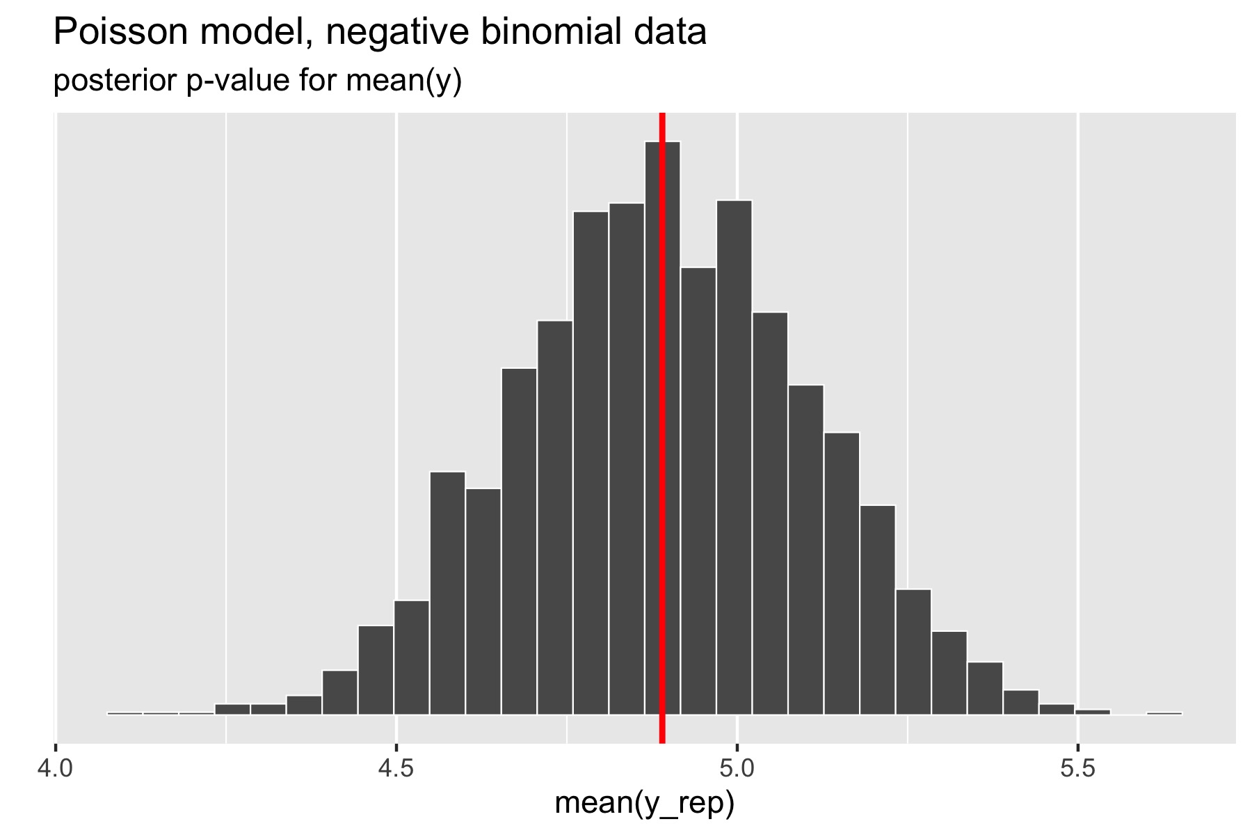
The p-value for the mean is just the percentage of replicated data sets whose statistic is greater than or equal that of the original data. Using a Poisson model for negative binomial data still fits the mean well, with a posterior $p$-value of 0.49. In Stan terms, it is extracted as the posterior mean of the indicator variable mean_gt.

The standard deviation statistic tells a different story.

Scatterplot of standard deviations of replicated data sets; the vertical red line is at standard deviation of original data.

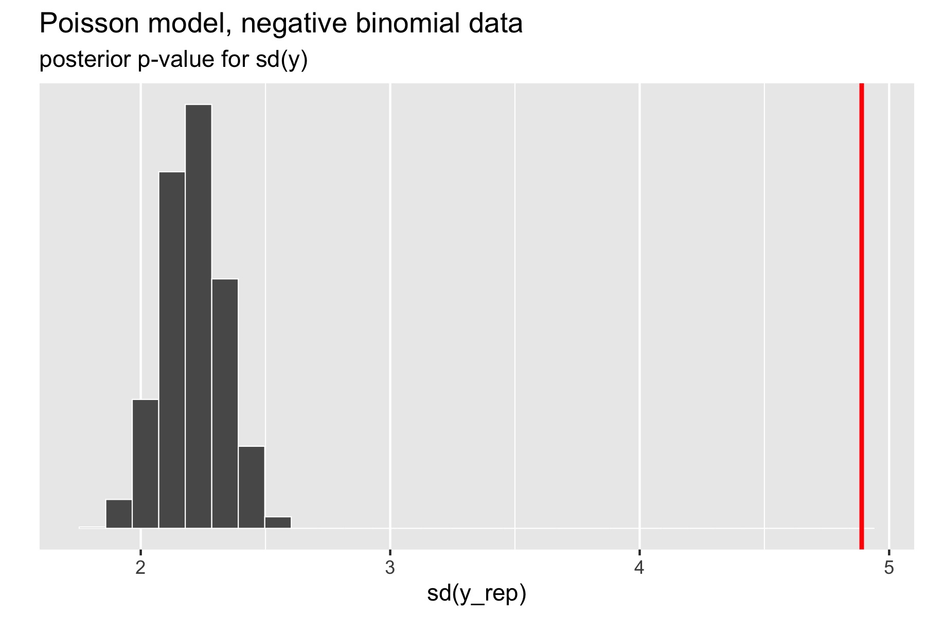
Here, the original data has much higher standard deviation than any of the replicated data sets. The resulting $p$-value estimated by Stan after a large number of iterations is exactly zero (the absolute error bounds are fine, but a lot of iterations are required to get good relative error bounds on small $p$-values by sampling). In other words, there were no posterior draws in which the replicated data set had a standard deviation greater than or equal to that of the original data set. Clearly, the model is not capturing the dispersion of the original data. The point of this exercise isn’t just to figure out that there’s a problem with a model, but to isolate where it is. Seeing that the data is over-dispersed compared to the Poisson model would be reason to fit a more general model like the negative binomial or a latent varying effects (aka random effects) model that can account for the over-dispersion.

Which statistics to test?

Any statistic may be used for the data, but these can be guided by the quantities of interest in the model itself. Popular choices in addition to mean and standard deviation are quantiles, such as the median, 5% or 95% quantiles, or even the maximum or minimum value to test extremes.

Despite the range of choices, test statistics should ideally be ancillary, in the sense that they should be testing something other than the fit of a parameter. For example, a simple normal model of a data set will typically fit the mean and variance of the data quite well as long as the prior doesn’t dominate the posterior. In contrast, a Poisson model of the same data cannot capture both the mean and the variance of a data set if they are different, so they bear checking in the Poisson case. As we saw with the Poisson case, the posterior mean for the single rate parameter was located near the data mean, not the data variance. Other distributions such as the lognormal and gamma distribution, have means and variances that are functions of two or more parameters.

Prior predictive checks

Prior predictive checks generate data according to the prior in order to asses whether a prior is appropriate (Gabry et al. 2019). A posterior predictive check generates replicated data according to the posterior predictive distribution. In contrast, the prior predictive check generates data according to the prior predictive distribution, $$y^{\text{sim}}\sim p(y).$$ The prior predictive distribution is just like the posterior predictive distribution with no observed data, so that a prior predictive check is nothing more than the limiting case of a posterior predictive check with no data.

This is easy to carry out mechanically by simulating parameters $${\theta }^{\text{sim}}\sim p(\theta )$$ according to the priors, then simulating data $$y^{\text{sim}}\sim p(y\mid {\theta }^{\text{sim}})$$ according to the data model given the simulated parameters. The result is a simulation from the joint distribution, $$(y^{\text{sim}},{\theta }^{\text{sim}})\sim p(y,\theta )$$ and thus $$y^{\text{sim}}\sim p(y)$$ is a simulation from the prior predictive distribution.

Coding prior predictive checks in Stan

A prior predictive check is coded just like a posterior predictive check. If a posterior predictive check has already been coded and it’s possible to set the data to be empty, then no additional coding is necessary. The disadvantage to coding prior predictive checks as posterior predictive checks with no data is that Markov chain Monte Carlo will be used to sample the parameters, which is less efficient than taking independent draws using random number generation.

Prior predictive checks can be coded entirely within the generated quantities block using random number generation. The resulting draws will be independent. Predictors must be read in from the actual data set—they do not have a generative model from which to be simulated. For a Poisson regression, prior predictive sampling can be encoded as the following complete Stan program.

data {
  int<lower=0> N;
  vector[N] x;
}
generated quantities {
  real alpha = normal_rng(0, 1);
  real beta = normal_rng(0, 1);
  array[N] real y_sim = poisson_log_rng(alpha + beta * x);
}

Running this program using Stan’s fixed-parameter sampler yields draws from the prior. These may be plotted to consider their appropriateness.

Example of prior predictive checks

Suppose we have a model for a football (aka soccer) league where there are $J$ teams. Each team has a scoring rate ${\lambda }_j$ and in each game will be assumed to score $\text{poisson}({\lambda }_j)$ points. Yes, this model completely ignores defense. Suppose the modeler does not want to “put their thumb on the scale” and would rather “let the data speak for themselves” and so uses a prior with very wide tails, because it seems uninformative, such as the widely deployed $${\lambda }_j\sim \text{gamma}({ϵ}_1,{ϵ}_2).$$ This is not just a manufactured example; The BUGS Book recommends setting $ϵ=(0.5,0.00001)$, which corresponds to a Jeffreys prior for a Poisson rate parameter prior (Lunn et al. 2012, 85).

Suppose the league plays a round-robin tournament wherein every team plays every other team. The following Stan model generates random team abilities and the results of such a round-robin tournament, which may be used to perform prior predictive checks.

data {
  int<lower=0> J;
  array[2] real<lower=0> epsilon;
}
generated quantities {
  array[J] real<lower=0> lambda;
  array[J, J] int y;
  for (j in 1:J) lambda[j] = gamma_rng(epsilon[1], epsilon[2]);
  for (i in 1:J) {
    for (j in 1:J) {
      y[i, j] = poisson_rng(lambda[i]) - poisson_rng(lambda[j]);
    }
  }
}

In this simulation, teams play each other twice and play themselves once. This could be made more realistic by controlling the combinatorics to only generate a single result for each pair of teams, of which there are $(\genfrac{}{}{0ex}{}{J}{2})=\frac{J\cdot (J-1)}{2}.$

Using the $\text{gamma}(0.5,0.00001)$ reference prior on team abilities, the following are the first 20 simulated point differences for the match between the first two teams, $y_{1,2}^{(1:20)}$.

2597 -26000   5725  22496   1270   1072   4502  -2809   -302   4987
7513   7527  -3268 -12374   3828   -158 -29889   2986  -1392     66

That’s some pretty highly scoring football games being simulated; all but one has a score differential greater than 100! In other words, this $\text{gamma}(0.5,0.00001)$ prior is putting around 95% of its weight on score differentials above 100. Given that two teams combined rarely score 10 points, this prior is way out of line with prior knowledge about football matches; it is not only consistent with outcomes that have never occurred in the history of the sport, it puts most of the prior probability mass there.

The posterior predictive distribution can be strongly affected by the prior when there is not much observed data and substantial prior mass is concentrated around infeasible values (A. Gelman 2006).

Just as with posterior predictive distributions, any statistics of the generated data may be evaluated. Here, the focus was on score difference between a single pair of teams, but it could’ve been on maximums, minimums, averages, variances, etc.

In this textbook example, the prior is univariate and directly related to the expected number of points scored, and could thus be directly inspected for consistency with prior knowledge about scoring rates in football. There will not be the same kind of direct connection when the prior and data model distributions are multivariate. In these more challenging situations, prior predictive checks are an easy way to get a handle on the implications of a prior in terms of what it says the data is going to look like; for a more complex application involving spatially heterogeneous air pollution concentration, see (Gabry et al. 2019).

Prior predictive checks can also be compared with the data, but one should not expect them to be calibrated in the same way as posterior predictive checks. That would require guessing the posterior and encoding it in the prior. The goal is make sure the prior is not so wide that it will pull probability mass away from feasible values.

Mixed predictive replication for hierarchical models

Andrew Gelman, Meng, and Stern (1996) discuss the case of mixed replication for hierarchical models in which the hyperparameters remain fixed, but varying effects are replicated. This is neither a purely prior nor purely posterior predictive check, but falls somewhere in between.

For example, consider a simple varying intercept logistic regression, with intercepts ${\alpha }_k$ for $k\in 1:K$. Each data item $y_n\in \{0,1\}$ is assumed to correspond to group $k{k}_n\in 1:K.$ The data model is thus $$y_n\sim \text{bernoulli}({\text{logit}}^{-1}({\alpha }_{kk[n]})).$$ The varying intercepts have a hierarchical normal prior, $${\alpha }_k\sim \text{normal}(\mu ,\sigma ).$$ The hyperparameters are themselves given weakly informative priors, $$\begin{array}{rcl}\mu & \sim & \text{normal}(0,2)\\ \sigma & \sim & \text{lognormal}(0,1).\end{array}$$

Like in a posterior predictive check, the hyperparameters $\mu$ and $\sigma$ are drawn from the posterior, $${\mu }^{(m)},{\sigma }^{(m)}\sim p(\mu ,\sigma \mid y)$$ Like in a prior predictive check, replicated values of $\alpha$ are drawn from the hyperparameters, $${\alpha }_k^{\text{rep}(m)}\sim \text{normal}({\alpha }_k\mid {\mu }^{(m)},{\sigma }^{(m)}).$$ The data items are then each replicated using the replicated intercepts, $$y_n^{\text{rep}(m)}\sim \text{bernoulli}({\text{logit}}^{-1}({\alpha }_{kk[n]}^{\text{rep}(m)})).$$ Thus the $y^{\text{rep}(m)}$ can be seen as a kind of posterior predictive replication of observations from new groups that were not among the original $K$ groups.

In Stan, mixed predictive replications $y^{\text{rep}(m)}$ can be programmed directly.

data {
  int<lower=0> K;
  int<lower=0> N;
  array[N] int<lower=1, upper=K> kk;
  array[N] int<lower=0, upper=1> y;
}
parameters {
  real mu;
  real<lower=0> sigma;
  vector<offset=mu, multiplier=sigma>[K] alpha;
}
model {
  mu ~ normal(0, 2);               // hyperprior
  sigma ~ lognormal(0, 1);
  alpha ~ normal(mu, sigma);       // hierarchical prior
  y ~ bernoulli_logit(alpha[kk]);  // data model
}
generated quantities {
  // alpha replicated;  mu and sigma not replicated
  array[K] real alpha_rep
    = normal_rng(rep_vector(mu, K), sigma);
  array[N] int<lower=0, upper=1> y_rep
    = bernoulli_logit_rng(alpha_rep[kk]);
}

Joint model representation

Following Andrew Gelman, Meng, and Stern (1996), prior, posterior, and mixed replications may all be defined as posteriors from joint models over parameters and observed and replicated data.

Posterior predictive model

For example, posterior predictive replication may be formulated using distribution notation as follows. $$\begin{array}{rcl}\theta & \sim & p(\theta )\\ y& \sim & p(y\mid \theta )\\ y^{\text{rep}}& \sim & p(y\mid \theta )\end{array}$$ The heavily overloaded distribution notation is meant to indicate that both $y$ and $y^{\text{rep}}$ are drawn from the same distribution, or more formally using capital letters to distinguish random variables, that the conditional densities $p_{Y^{\text{rep}}\mid \mathrm{\Theta }}$ and $p_{Y\mid \mathrm{\Theta }}$ are the same.

The joint density is $$p(\theta ,y,y^{\text{rep}})=p(\theta )\cdot p(y\mid \theta )\cdot p(y^{\text{rep}}\mid \theta ).$$ This again is assuming that the two distributions for $y$ and $y^{\text{rep}}$ are identical.

The variable $y$ is observed, with the predictive simulation $y^{\text{rep}}$ and parameter vector $\theta$ not observed. The posterior is $p(y^{\text{rep}},\theta \mid y)$. Given draws from the posterior, the posterior predictive simulations $y^{\text{rep}}$ are retained.

Prior predictive model

The prior predictive model simply drops the data component of the posterior predictive model. $$\begin{array}{rcl}\theta & \sim & p(\theta )\\ y^{\text{rep}}& \sim & p(y\mid \theta )\end{array}$$ This corresponds to the joint density $$p(\theta ,y^{\text{rep}})=p(\theta )\cdot p(y^{\text{rep}}\mid \theta ).$$

It is typically straightforward to draw $\theta$ from the prior and $y^{\text{rep}}$ from the data model given $\theta$ efficiently. In cases where it is not, the model may be coded and executed just as the posterior predictive model, only with no data.

Mixed replication for hierarchical models

The mixed replication corresponds to the model $$\begin{array}{rcl}\varphi & \sim & p(\varphi )\\ \alpha & \sim & p(\alpha \mid \varphi )\\ y& \sim & p(y\mid \alpha )\\ {\alpha }^{\text{rep}}& \sim & p(\alpha \mid \varphi )\\ y^{\text{rep}}& \sim & p(y\mid \varphi )\end{array}$$ The notation here is meant to indicate that $\alpha$ and ${\alpha }^{\text{rep}}$ have identical distributions, as do $y$ and $y^{\text{rep}}$.

This corresponds to a joint model $$p(\varphi ,\alpha ,{\alpha }^{\text{rep}},y,y^{\text{rep}})=p(\varphi )\cdot p(\alpha \mid \varphi )\cdot p(y\mid \alpha )\cdot p({\alpha }^{\text{rep}}\mid \varphi )\cdot p(y^{\text{rep}}\mid {\alpha }^{\text{rep}}),$$ where $y$ is the only observed variable, $\alpha$ contains the lower-level parameters and $\varphi$ the hyperparameters. Note that $\varphi$ is not replicated and instead appears in the distribution for both $\alpha$ and ${\alpha }^{\text{rep}}$.

The posterior is $p(\varphi ,\alpha ,{\alpha }^{\text{rep}},y^{\text{rep}}\mid y)$. From posterior draws, the posterior predictive simulations $y^{\text{rep}}$ are kept.

References

Bayarri, MJ, and James O Berger. 2000. “P Values for Composite Null Models.” Journal of the American Statistical Association 95 (452): 1127–42.

Gabry, Jonah, Daniel Simpson, Aki Vehtari, Michael Betancourt, and Andrew Gelman. 2019. “Visualization in Bayesian Workflow.” Journal of the Royal Statistical Society: Series A (Statistics in Society) 182 (2): 389–402.

Gelman, A. 2006. “Prior Distributions for Variance Parameters in Hierarchical Models.” Bayesian Analysis 1 (3): 515–34.

Gelman, Andrew, Xiao-Li Meng, and Hal Stern. 1996. “Posterior Predictive Assessment of Model Fitness via Realized Discrepancies.” Statistica Sinica, 733–60.

Lunn, David, Christopher Jackson, Nicky Best, Andrew Thomas, and David Spiegelhalter. 2012. The BUGS Book: A Practical Introduction to Bayesian Analysis. CRC Press/Chapman & Hall.

Rubin, Donald B. 1984. “Bayesianly Justifiable and Relevant Frequency Calculations for the Applied Statistician.” The Annals of Statistics, 1151–72.