Simulation-Based Calibration Checking
A Bayesian posterior is calibrated if the posterior intervals have appropriate coverage. For example, 80% intervals are expected to contain the true parameter 80% of the time. If data is generated according to a model, Bayesian posterior inference with respect to that model is calibrated by construction. Simulation-based calibration checking (SBC) exploits this property of Bayesian inference to assess the soundness of a posterior sampler. Roughly, the way it works is by simulating parameters according to the prior, then simulating data conditioned on the simulated parameters, then testing posterior calibration of the inference algorithm over independently simulated data sets. This chapter follows Talts et al. (2018), which improves on the original approach developed by Cook, Gelman, and Rubin (2006). See also Modrák et al. (2023) for further improvements.
Bayes is calibrated by construction
Suppose a Bayesian model is given in the form of a prior density \(p(\theta)\) and sampling density \(p(y \mid \theta).\) Now consider a process that first simulates parameters from the prior, \[ \theta^{\textrm{sim}} \sim p(\theta), \] and then simulates data given the parameters, \[ y^{\textrm{sim}} \sim p(y \mid \theta^{\textrm{sim}}). \] By the definition of conditional densities, the simulated data and parameters constitute an independent draw from the model’s joint distribution, \[ (y^{\textrm{sim}}, \theta^{\textrm{sim}}) \sim p(y, \theta). \] From Bayes’s rule, it follows that for any observed (fixed) data \(y\), \[ p(\theta \mid y) \propto p(y, \theta). \] Therefore, the simulated parameters constitute a draw from the posterior for the simulated data, \[ \theta^{\textrm{sim}} \sim p(\theta \mid y^{\textrm{sim}}). \] Now consider an algorithm that produces a sequence of draws from the posterior given this simulated data, \[ \theta^{(1)}, \ldots, \theta^{(M)} \sim p(\theta \mid y^{\textrm{sim}}). \] Because \(\theta^{\textrm{sim}}\) is also distributed as a draw from the posterior, the rank statistics of \(\theta^{\textrm{sim}}\) with respect to \(\theta^{(1)}, \ldots \theta^{(M)}\) should be uniform.
This is one way to define calibration, because it follows that posterior intervals will have appropriate coverage (Dawid 1982; Gneiting, Balabdaoui, and Raftery 2007). If the rank of \(\theta^{\textrm{sim}}\) is uniform among the draws \(\theta^{(1)}, \ldots, \theta^{(M)},\) then for any 90% interval selected, the probability the true value \(\theta^{\textrm{sim}}\) falls in it will also be 90%. The same goes for any other posterior interval.
Simulation-based calibration checking
Suppose the Bayesian model to test has joint density \[ p(y, \theta) = p(y \mid \theta) \cdot p(\theta), \] with data \(y\) and parameters \(\theta\) (both are typically multivariate). Simulation-based calibration checking works by generating \(N\) simulated parameter and data pairs according to the joint density, \[ (y^{\textrm{sim}(1)}, \theta^{\textrm{sim}(1)}), \ldots, (y^{\textrm{sim}(N)}, \theta^{\textrm{sim}(N)}), \sim p(y, \theta). \] For each simulated data set \(y^{\textrm{sim}(n)}\), use the algorithm to be tested to generate \(M\) posterior draws, which if everything is working properly, will be distributed marginally as \[ \theta^{(n, 1)}, \ldots, \theta^{(n, M)} \sim p(\theta \mid y^{\textrm{sim}(n)}). \] For a simulation \(n\) and parameter \(k\), the rank of the simulated parameter among the posterior draws is \[\begin{eqnarray*} r_{n, k} & = & \textrm{rank}(\theta_k^{\textrm{sim}(n)}, (\theta^{(n, 1)}, \ldots, \theta^{(n,M)})) \\[4pt] & = & \sum_{m = 1}^M \textrm{I}[\theta_k^{(n,m)} < \theta_k^{\textrm{sim}(n)}]. \end{eqnarray*}\] That is, the rank is the number of posterior draws \(\theta^{(n,m)}_k\) that are less than the simulated draw \(\theta^{\textrm{sim}(n)}_k.\)
If the algorithm generates posterior draws according to the posterior, the ranks should have uniform discrete distribution from \(0\) to \(M\), so that the ranks plus one are uniformly distributed from \(1\) to \(M + 1\), \[ r_{n, k} + 1 \sim \textrm{categorical}\! \left(\frac{1}{M + 1}, \ldots, \frac{1}{M + 1}\right). \] Simulation-based calibration checking uses this expected behavior to test the calibration of each parameter of a model on simulated data. Talts et al. (2018) suggest plotting binned counts of \(r_{1:N, k}\) for different parameters \(k\); Säilynoja, Bürkner, and Vehtari (2022) provide a graphical test for discrete uniformity testing. Before uniformity testing the Markov chains should be thinned to remove autocorrelation as these uniformity tests assume independence (Säilynoja, Bürkner, and Vehtari 2022).
SBC in Stan
Running simulation-based calibration checking in Stan will test whether Stan’s sampling algorithm can sample from the posterior associated with data generated according to the model. The data simulation and posterior fitting and rank calculation can all be done within a single Stan program. Then Stan’s posterior sampler has to be run multiple times. Each run produces a rank for each parameter being assessed for uniformity. The total set of ranks can then be tested for uniformity.
Example model
For illustration, a very simple model will suffice. Suppose there are two parameters \((\mu, \sigma)\) with independent priors, \[ \mu \sim \textrm{normal}(0, 1), \] and \[ \sigma \sim \textrm{lognormal}(0, 1). \] The data \(y = y_1, \ldots, y_N\) is drawn conditionally independently given the parameters, \[ y_n \sim \textrm{normal}(\mu, \sigma). \] The joint prior density is thus \[ p(\mu, \sigma) = \textrm{normal}(\mu \mid 0, 1) \cdot \textrm{lognormal}(\sigma \mid 0, 1), \] and the data model is \[ p(y \mid \mu, \sigma) = \prod_{n=1}^N \textrm{normal}(y_n \mid \mu, \sigma). \]
For example, suppose the following two parameter values are drawn from the prior in the first simulation, \[ (\mu^{\textrm{sim(1)}}, \sigma^{\textrm{sim(1)}}) = (1.01, 0.23). \] Then data \(y^{\textrm{sim}(1)} \sim p(y \mid \mu^{\textrm{sim(1)}}, \sigma^{\textrm{sim(1)}})\) is drawn according to the data model. Next, \(M = 4\) draws are taken from the posterior \(\mu^{(1,m)}, \sigma^{(1,m)} \sim p(\mu, \sigma \mid y^{\textrm{sim}(1)})\), \[ \begin{array}{r|rr} m & \mu^{(1,m)} & \sigma^{(1,m)} \\ \hline 1 & 1.07 & 0.33 \\ 2 & -0.32 & 0.14 \\ 3 & -0.99 & 0.26 \\ 4 & 1.51 & 0.31 \end{array} \] Then the comparisons on which ranks are based look as follows, \[ \begin{array}{r|cc} m & \textrm{I}(\mu^{(1,m)} < \mu^{\textrm{sim}(1)}) & \textrm{I}(\sigma^{(1,m)} < \sigma^{\textrm{sim}(1)}) \\ \hline 1 & 0 & 0 \\ 2 & 1 & 1 \\ 3 & 1 & 0 \\ 4 & 0 & 0 \end{array} \] The ranks are the column sums, \(r_{1,1} = 2\) and \(r_{1,2} = 1\). Because the simulated parameters are distributed according to the posterior, these ranks should be distributed uniformly between \(0\) and \(M\), the number of posterior draws.
Testing a Stan program with simulation-based calibration checking
To code simulation-based calibration checking in a Stan program, the transformed data block can be used to simulate parameters and data from the model. The parameters, transformed parameters, and model block then define the model over the simulated data. Then, in the generated quantities block, the program records an indicator for whether each parameter is less than the simulated value. As shown above, the rank is then the sum of the simulated indicator variables.
transformed data {
  real mu_sim = normal_rng(0, 1);
  real<lower=0> sigma_sim = lognormal_rng(0, 1);
  int<lower=0> J = 10;
  vector[J] y_sim;
  for (j in 1:J) {
    y_sim[j] = normal_rng(mu_sim, sigma_sim);
  }
}
parameters {
  real mu;
  real<lower=0> sigma;
}
model {
  mu ~ normal(0, 1);
  sigma ~ lognormal(0, 1);
  y_sim ~ normal(mu, sigma);
}
generated quantities {
  array[2] int<lower=0, upper=1> lt_sim
      = { mu < mu_sim, sigma < sigma_sim };
}
To avoid confusion with the number of simulated data sets used for simulation-based calibration checking, J is used for the number of simulated data points.
The model is implemented twice—once as a data generating process using random number generators in the transformed data block, then again in the parameters and model block. This duplication is a blessing and a curse. The curse is that it’s more work and twice the chance for errors. The blessing is that by implementing the model twice and comparing results, the chance of there being a mistake in the model is reduced.
Pseudocode for simulation-based calibration checking
The entire simulation-based calibration checking process is as follows, where
p(theta)is the prior densityp(y | theta)is the sampling densityKis the number of parametersNis the total number of simulated data sets and fitsMis the number of posterior draws per simulated data set
SBC(p(theta), p(y | theta), K, N, M)
------------------------------------
for (n in 1:N) {
    // simulate parameters and data
    theta(sim(n)) ~ p(theta)
    y(sim(n)) ~ p(y | theta(sim(n)))

    // posterior draws given simulated data
    for (m in 1:M) {
        theta(n, m) ~ p(theta | y(sim(n)))
    }
    // calculate rank of sim among posterior draws
    for (k in 1:K) {
        rank(n, k) = SUM_m I(theta[k](n,m) < theta[k](sim(n)))
    }
}
// test uniformity of each parameter
for (k in 1:K) {
    test uniformity of rank(1:N, k)
}
The importance of thinning
The draws from the posterior are assumed to be roughly independent. If they are not, artifacts may arise in the uniformity tests due to correlation in the posterior draws (Säilynoja, Bürkner, and Vehtari 2022). Thus it is best to thin the posterior draws down to the point where the effective sample size is roughly the same as the number of thinned draws. This may require running the code a few times to judge the number of draws required to produce a target effective sample size. This operation that can be put into a loop that doubles the number of iterations until all parameters have an effective sample size of M, then thinning down to M draws.
Testing uniformity
A simple, though not very highly powered, \(\chi^2\)-squared test for uniformity can be formulated by binning the ranks \(0:M\) into \(J\) bins and testing that the bins all have roughly the expected number of draws in them. Many other tests for uniformity are possible. For example, Säilynoja, Bürkner, and Vehtari (2022) use binomial model pointiwise for the empirical cumlative distribution function and adjust to obtain simulatenous envelope to be used as graphical uniformity test.
The bins don’t need to be exactly the same size. In general, if \(b_j\) is the number of ranks that fall into bin \(j\) and \(e_j\) is the number of ranks expected to fall into bin \(j\) (which will be proportional to its size under uniformity), the test statistic is \[ X^2 = \sum_{j = 1}^J \frac{(b_j - e_j)^2}{e_j}. \] The terms are approximately square standard normal, so that under the null hypothesis of uniformity, \[ X^2 \sim \textrm{chiSquared}(J - 1), \] with the corresponding \(p\)-value given by the complementary cumulative distribution function (CCDF) of \(\textrm{chiSquared}(J - 1)\) applied to \(X^2\). Because this test relies on the binomial being approximately normal, the traditional advice is to make sure the expected count in each bin is at least five, i.e., \(e_j \geq 5.\)
Indexing to simplify arithmetic
Because there are \(M + 1\) possible ranks, with \(J\) bins, it is easiest to have \(M + 1\) be divisible by \(J\). For instance, if \(J = 20\) and \(M = 999\), then there are \(1000\) possible ranks and an expected count in each bin of \(\frac{M + 1}{J} = 50.\)
Distributing the ranks into bins is another fiddly operation that can be done with integer arithmetic or the floor operation. Using floor, the following function determines the bin for a rank, \[ \textrm{bin}(r_{n, m}, M, J) = 1 + \left\lfloor \frac{r_{n, m}}{(M + 1) / J} \right\rfloor. \] For example, with \(M = 999\) and \(J = 20\), \((M + 1) / J = 50\). The lowest rank checks out, \[ \textrm{bin}(0, 999, 20) = 1 + \lfloor 0 / 50 \rfloor = 1, \] as does the 50th rank, \[ \textrm{bin}(49, 999, 20) = 1 + \lfloor 49 / 50 \rfloor = 1, \] and the 51st is appropriately put in the second bin, \[ \textrm{bin}(50, 999, 20) = 1 + \lfloor 50 / 50 \rfloor = 2. \] The highest rank also checks out, with \(\textrm{bin}(1000, 999, 20) = 50.\)
To summarize, the following pseudocode computes the \(b_j\) values for the \(\chi^2\) test or for visualization in a histogram.
Inputs: M draws, J bins, N parameters, ranks r[n, m]
b[1:J] = 0
for (m in 1:M) {
  ++b[1 + floor(r[n, m] * J / (M + 1))]
}
where the ++b[n] notation is a common form of syntactic sugar for b[n] = b[n] + 1.
In general, a great deal of care must be taken in visualizing discrete data because it’s easy to introduce off-by-one errors and artifacts at the edges because of the way boundaries are computed by default. That’s why so much attention must be devoted to indexing and binning.
Examples of simulation-based calibration checking
This section will show what the results look like when the tests pass and then when they fail. The passing test will compare a normal model and normal data generating process, whereas the second will compare a normal model with a Student-t data generating process. The first will produce calibrated posteriors, the second will not.
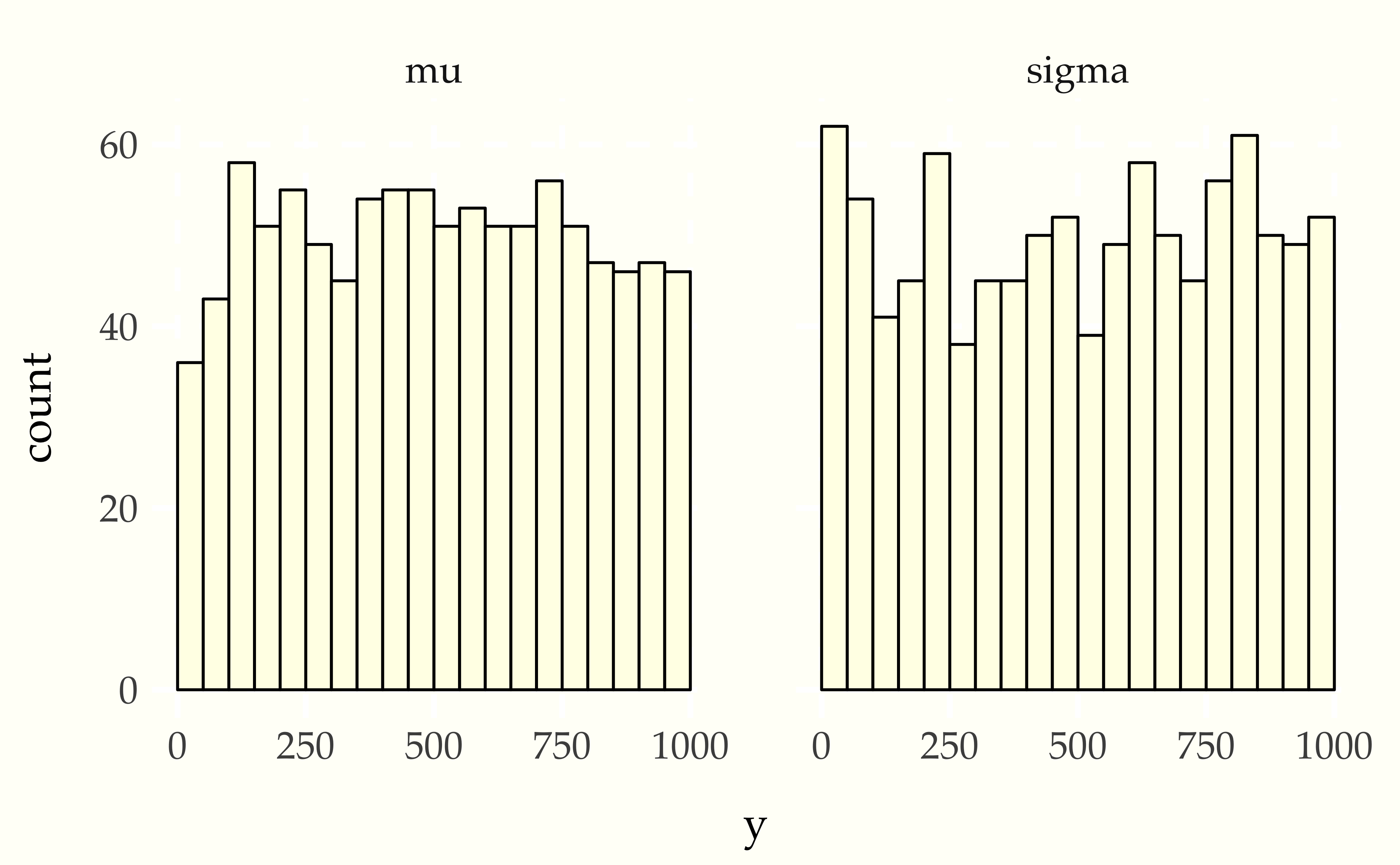
When things go right
Consider the following simple model for a normal distribution with standard normal and lognormal priors on the location and scale parameters. \[\begin{eqnarray*} \mu & \sim & \textrm{normal}(0, 1) \\[4pt] \sigma & \sim & \textrm{lognormal}(0, 1) \\[4pt] y_{1:10} & \sim & \textrm{normal}(\mu, \sigma). \end{eqnarray*}\] The Stan program for evaluating SBC for this model is
transformed data {
  real mu_sim = normal_rng(0, 1);
  real<lower=0> sigma_sim = lognormal_rng(0, 1);

  int<lower=0> J = 10;
  vector[J] y_sim;
  for (j in 1:J) {
    y_sim[j] = student_t_rng(4, mu_sim, sigma_sim);
  }
}
parameters {
  real mu;
  real<lower=0> sigma;
}
model {
  mu ~ normal(0, 1);
  sigma ~ lognormal(0, 1);

  y_sim ~ normal(mu, sigma);
}
generated quantities {
  array[2] int<lower=0, upper=1> I_lt_sim
      = { mu < mu_sim, sigma < sigma_sim };
}
After running this for enough iterations so that the effective sample size is larger than \(M\), then thinning to \(M\) draws (here \(M = 999\)), the ranks are computed and binned, and then plotted.
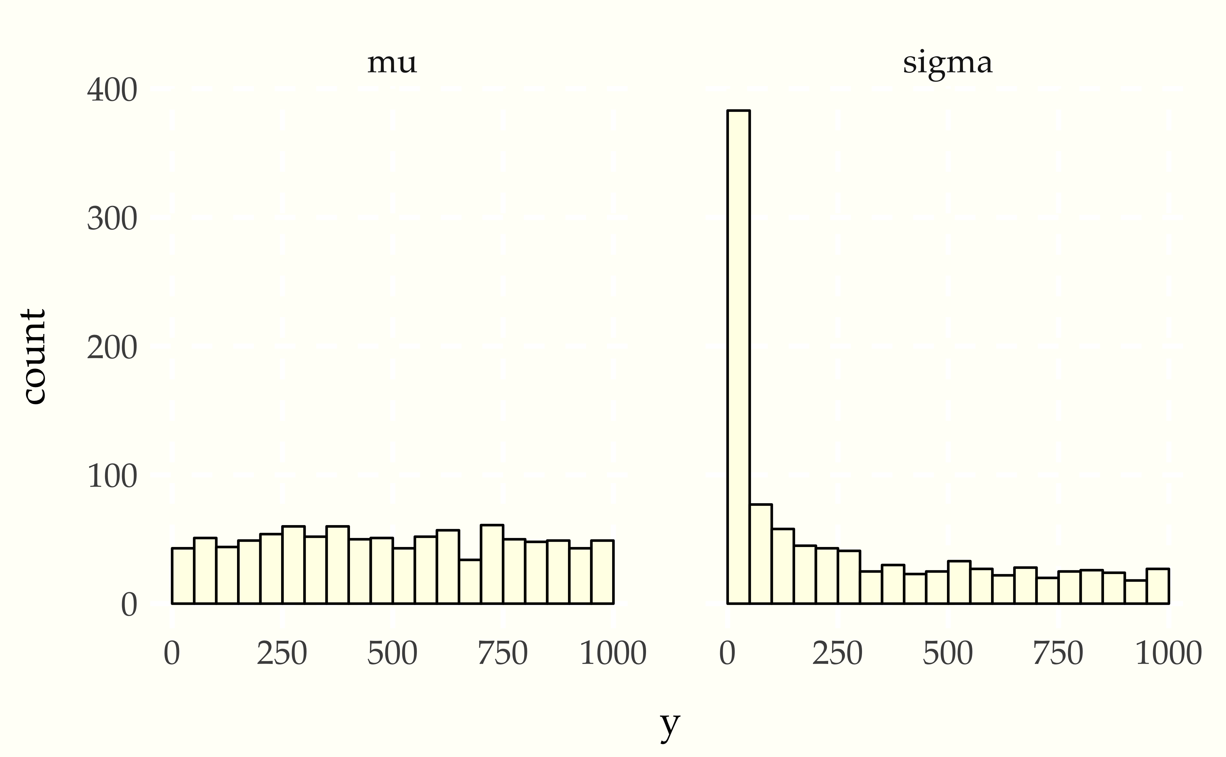
When things go wrong
Now consider using a Student-t data generating process with a normal model. Compare the apparent uniformity of the well specified model with the ill-specified situation with Student-t generative process and normal model.
When Stan’s sampler goes wrong
The example in the previous sections show hard-coded pathological behavior. The usual application of SBC is to diagnose problems with a sampler.
This can happen in Stan with well-specified models if the posterior geometry is too difficult (usually due to extreme stiffness that varies). A simple example is the eight schools problem, the data for which consists of sample means \(y_j\) and standard deviations \(\sigma_j\) of differences in test score after the same intervention in \(J = 8\) different schools. Rubin (1981) applies a hierarchical model for a meta-analysis of the results, estimating the mean intervention effect and a varying effect for each school. With a standard parameterization and weak priors, this model has very challenging posterior geometry, as shown by Talts et al. (2018); this section replicates their results.
The meta-analysis model has parameters for a population mean \(\mu\) and standard deviation \(\tau > 0\) as well as the effect \(\theta_j\) of the treatment in each school. The model has weak normal and half-normal priors for the population-level parameters, \[\begin{eqnarray*} \mu & \sim & \textrm{normal}(0, 5) \\[4pt] \tau & \sim & \textrm{normal}_{+}(0, 5). \end{eqnarray*}\] School level effects are modeled as normal given the population parameters, \[ \theta_j \sim \textrm{normal}(\mu, \tau). \] The data is modeled as in a meta-analysis, given the school effect and sample standard deviation in the school, \[ y_j \sim \textrm{normal}(\theta_j, \sigma_j). \]
This model can be coded in Stan with a data-generating process that simulates the parameters and then simulates data according to the parameters.
transformed data {
  real mu_sim = normal_rng(0, 5);
  real tau_sim = abs(normal_rng(0, 5));
  int<lower=0> J = 8;
  array[J] real theta_sim = normal_rng(rep_vector(mu_sim, J), tau_sim);
  array[J] real<lower=0> sigma = abs(normal_rng(rep_vector(0, J), 5));
  array[J] real y = normal_rng(theta_sim, sigma);
}
parameters {
  real mu;
  real<lower=0> tau;
  array[J] real theta;
}
model {
  tau ~ normal(0, 5);
  mu ~ normal(0, 5);
  theta ~ normal(mu, tau);
  y ~ normal(theta, sigma);
}
generated quantities {
  int<lower=0, upper=1> mu_lt_sim = mu < mu_sim;
  int<lower=0, upper=1> tau_lt_sim = tau < tau_sim;
  int<lower=0, upper=1> theta1_lt_sim = theta[1] < theta_sim[1];
}
As usual for simulation-based calibration checking, the transformed data encodes the data-generating process using random number generators. Here, the population parameters \(\mu\) and \(\tau\) are first simulated, then the school-level effects \(\theta\), and then finally the observed data \(\sigma_j\) and \(y_j.\) The parameters and model are a direct encoding of the mathematical presentation using vectorized sampling statements. The generated quantities block includes indicators for parameter comparisons, saving only \(\theta_1\) because the schools are exchangeable in the simulation.
When fitting the model in Stan, multiple warning messages are provided that the sampler has diverged. The divergence warnings are in Stan’s sampler precisely to diagnose the sampler’s inability to follow the curvature in the posterior and provide independent confirmation that Stan’s sampler cannot fit this model as specified.
SBC also diagnoses the problem. Here’s the rank plots for running \(N = 200\) simulations with 1000 warmup iterations and \(M = 999\) draws per simulation used to compute the ranks.
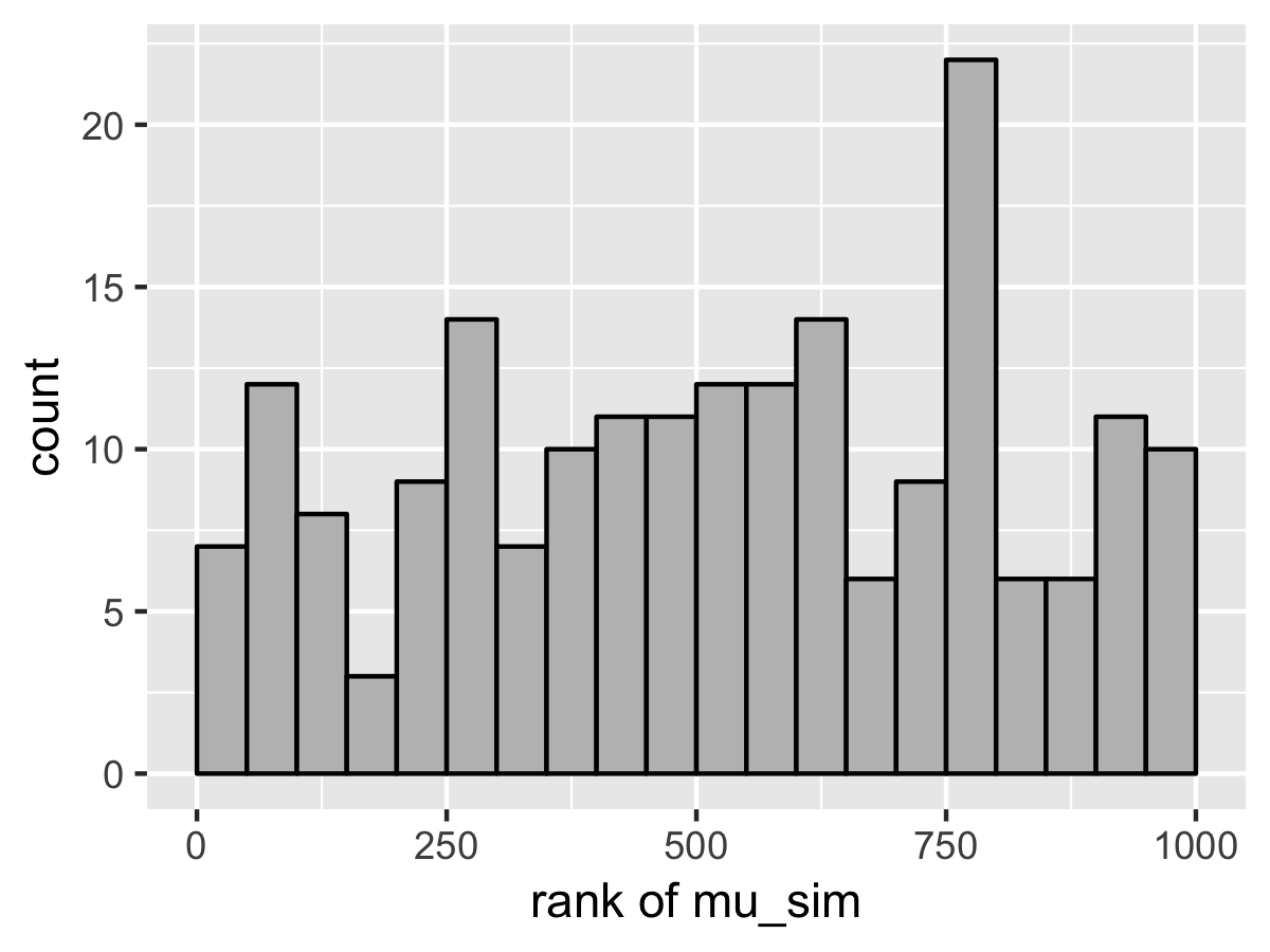
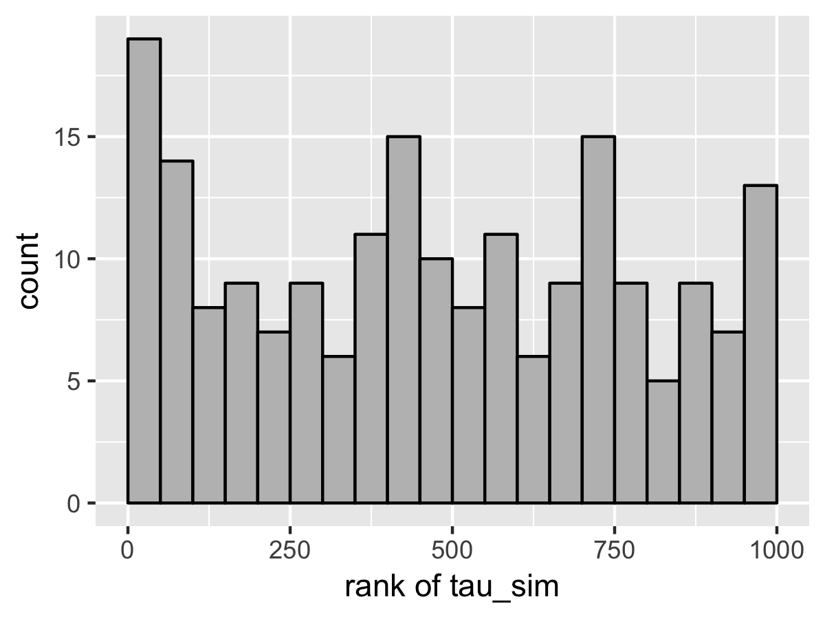
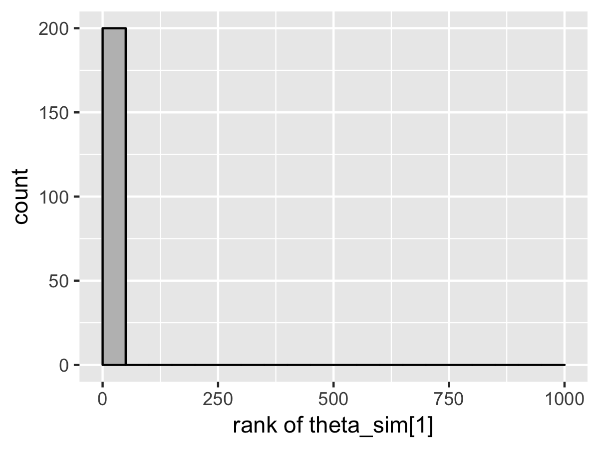
Although the population mean and standard deviation \(\mu\) and \(\tau\) appear well calibrated, \(\theta_1\) tells a very different story. The simulated values are much smaller than the values fit from the data. This is because Stan’s no-U-turn sampler is unable to sample with the model formulated in the centered parameterization—the posterior geometry has regions of extremely high curvature as \(\tau\) approaches zero and the \(\theta_j\) become highly constrained. The chapter on reparameterization explains how to remedy this problem and fit this kind of hierarchical model with Stan.