25.5 Examples of simulation-based calibration
This section will show what the results look like when the tests pass and then when they fail. The passing test will compare a normal model and normal data generating process, whereas the second will compare a normal model with a Student-t data generating process. The first will produce calibrated posteriors, the second will not.
25.5.1 When things go right
Consider the following simple model for a normal distribution with standard normal and lognormal priors on the location and scale parameters. \[\begin{eqnarray*} \mu & \sim & \textrm{normal}(0, 1) \\[4pt] \sigma & \sim & \textrm{lognormal}(0, 1) \\[4pt] y_{1:10} & \sim & \textrm{normal}(\mu, \sigma). \end{eqnarray*}\] The Stan program for evaluating SBC for this model is
transformed data {
  real mu_sim = normal_rng(0, 1);
  real<lower = 0> sigma_sim = lognormal_rng(0, 1);

  int<lower = 0> J = 10;
  vector[J] y_sim;
  for (j in 1:J)
    y_sim[j] = student_t_rng(4, mu_sim, sigma_sim);
}
parameters {
  real mu;
  real<lower = 0> sigma;
}
model {
  mu ~ normal(0, 1);
  sigma ~ lognormal(0, 1);

  y_sim ~ normal(mu, sigma);
}
generated quantities {
  int<lower = 0, upper = 1> I_lt_sim[2]
      = { mu < mu_sim, sigma < sigma_sim };
}
After running this for enough iterations so that the effective sample size is larger than \(M\), then thinning to \(M\) draws (here \(M = 999\)), the ranks are computed and binned, and then plotted.
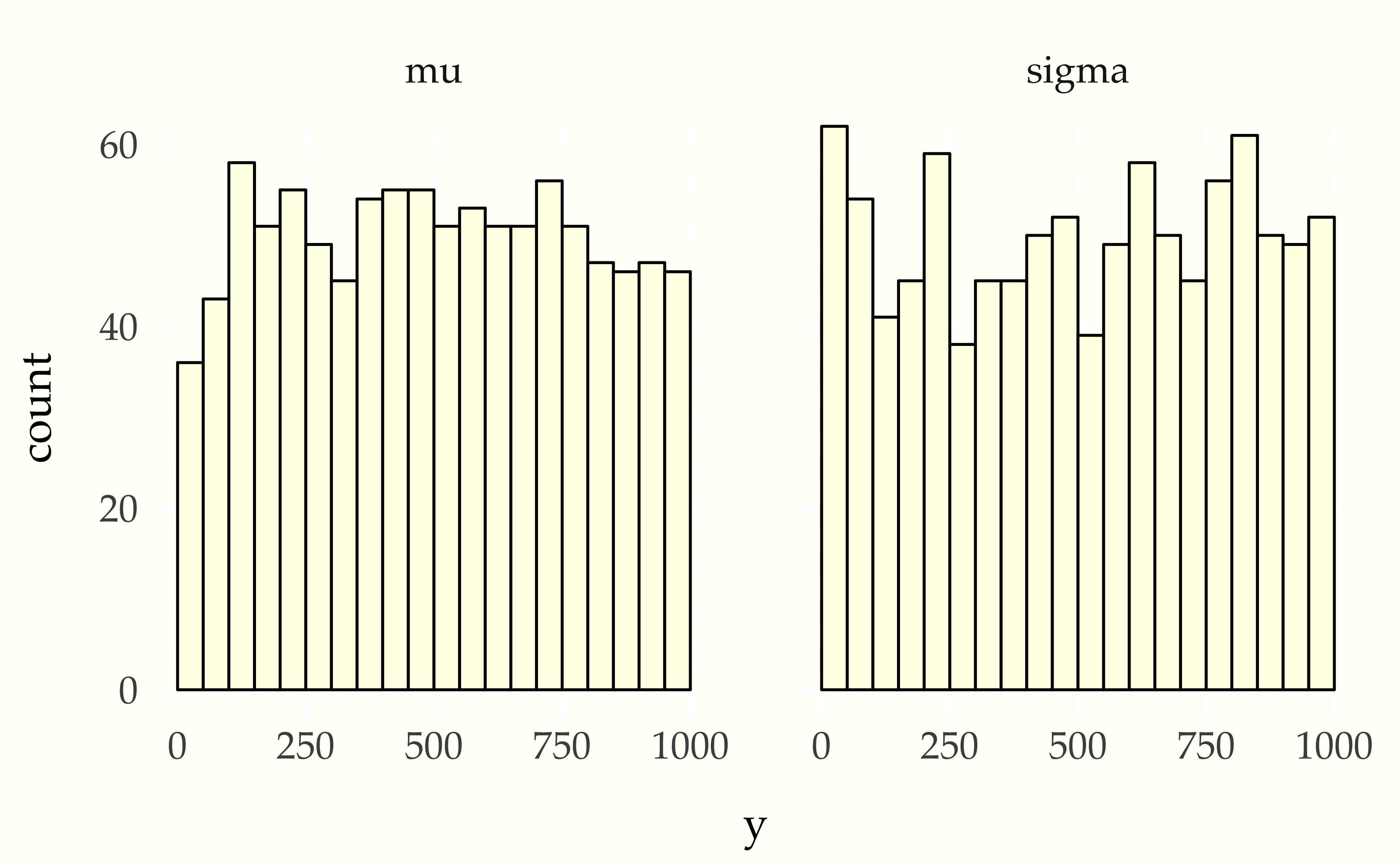
Figure 25.1: Simulation based calibration plots for location and scale of a normal model with standard normal prior on the location standard lognormal prior on the scale. Both histograms appear uniform, which is consistent with inference being well calibrated.
25.5.2 When things go wrong
Now consider using a Student-t data generating process with a normal model. Compare the apparent uniformity of the well specified model with the ill-specified situation with Student-t generative process and normal model.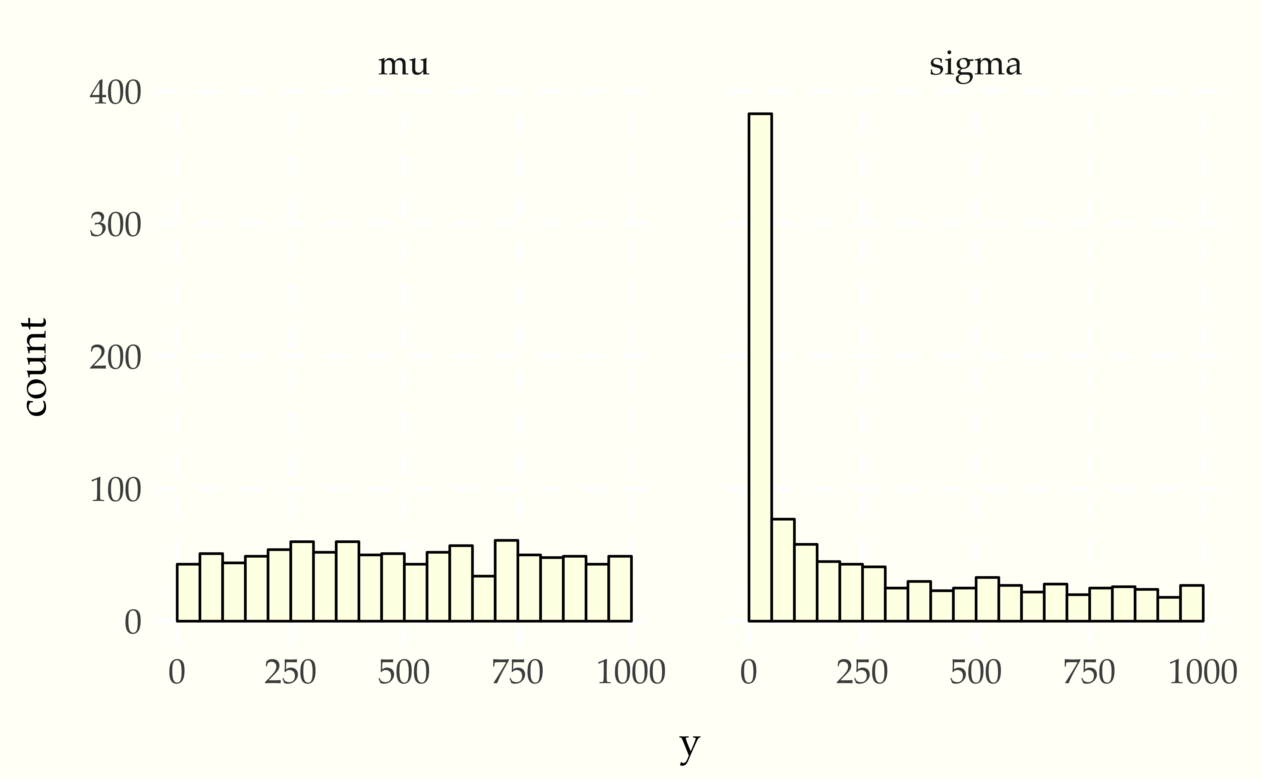
Figure 25.2: Simulation based calibration plots for location and scale of a normal model with standard normal prior on the location standard lognormal prior on the scale with mismatched generative model using a Student-t likelihood with 4 degrees of freedom. The mean histogram appears uniform, but the scale parameter shows simulated values much smaller than fit values, clearly signaling the lack of calibration.
25.5.3 When Stan’s sampler goes wrong
The example in the previous sections show hard-coded pathological behavior. The usual application of SBC is to diagnose problems with a sampler.
This can happen in Stan with well-specified models if the posterior geometry is too difficult (usually due to extreme stiffness that varies). A simple example is the eight schools problem, the data for which consists of sample means \(y_j\) and standard deviations \(\sigma_j\) of differences in test score after the same intervention in \(J = 8\) different schools. Rubin (1981) applies a hierarchical model for a meta-analysis of the results, estimating the mean intervention effect and a varying effect for each school. With a standard parameterization and weak priors, this model has very challenging posterior geometry, as shown by Talts et al. (2018); this section replicates their results.
The meta-analysis model has parameters for a population mean \(\mu\) and standard deviation \(\tau > 0\) as well as the effect \(\theta_j\) of the treatment in each school. The model has weak normal and half-normal priors for the population-level parameters, \[\begin{eqnarray*} \mu & \sim & \textrm{normal}(0, 5) \\[4pt] \tau & \sim & \textrm{normal}_{+}(0, 5). \end{eqnarray*}\] School level effects are modeled as normal given the population parameters, \[ \theta_j \sim \textrm{normal}(\mu, \tau). \] The data is modeled as in a meta-analysis, given the school effect and sample standard deviation in the school, \[ y_j \sim \textrm{normal}(\theta_j, \sigma_j). \]
This model can be coded in Stan with a data-generating process that simulates the parameters and then simulates data according to the parameters.
transformed data {
  real mu_sim = normal_rng(0, 5);
  real tau_sim = fabs(normal_rng(0, 5));
  int<lower = 0> J = 8;
  real theta_sim[J] = normal_rng(rep_vector(mu_sim, J), tau_sim);
  real<lower=0> sigma[J] = fabs(normal_rng(rep_vector(0, J), 5));
  real y[J] = normal_rng(theta_sim, sigma);
}
parameters {
  real mu;
  real<lower=0> tau;
  real theta[J];
}
model {
  tau ~ normal(0, 5);
  mu ~ normal(0, 5);
  theta ~ normal(mu, tau);
  y ~ normal(theta, sigma);
}
generated quantities {
  int<lower = 0, upper = 1> mu_lt_sim = mu < mu_sim;
  int<lower = 0, upper = 1> tau_lt_sim = tau < tau_sim;
  int<lower = 0, upper = 1> theta1_lt_sim = theta[1] < theta_sim[1];
}
As usual for simulation-based calibration, the transformed data encodes the data-generating process using random number generators. Here, the population parameters \(\mu\) and \(\tau\) are first simulated, then the school-level effects \(\theta\), and then finally the observed data \(\sigma_j\) and \(y_j.\) The parameters and model are a direct encoding of the mathematical presentation using vectorized sampling statements. The generated quantities block includes indicators for parameter comparisons, saving only \(\theta_1\) because the schools are exchangeable in the simulation.
When fitting the model in Stan, multiple warning messages are provided that the sampler has diverged. The divergence warnings are in Stan’s sampler precisely to diagnose the sampler’s inability to follow the curvature in the posterior and provide independent confirmation that Stan’s sampler cannot fit this model as specified.
SBC also diagnoses the problem. Here’s the rank plots for running \(N = 200\) simulations with 1000 warmup iterations and \(M = 999\) draws per simulation used to compute the ranks.
![Simulation based calibration plots for the eight-schools model with centered parameterization in Stan. The geometry is too difficult for the NUTS sampler to handle, as indicated by the plot for theta[1].](img/sbc-ctr-8-schools-mu.png)
![Simulation based calibration plots for the eight-schools model with centered parameterization in Stan. The geometry is too difficult for the NUTS sampler to handle, as indicated by the plot for theta[1].](img/sbc-ctr-8-schools-tau.png)
![Simulation based calibration plots for the eight-schools model with centered parameterization in Stan. The geometry is too difficult for the NUTS sampler to handle, as indicated by the plot for theta[1].](img/sbc-ctr-8-schools-theta1.png)
Figure 25.3: Simulation based calibration plots for the eight-schools model with centered parameterization in Stan. The geometry is too difficult for the NUTS sampler to handle, as indicated by the plot for theta[1].
Although the population mean and standard deviation \(\mu\) and \(\tau\) appear well calibrated, \(\theta_1\) tells a very different story. The simulated values are much smaller than the values fit from the data. This is because Stan’s no-U-turn sampler is unable to sample with the model formulated in the centered parameterization—the posterior geometry has regions of extremely high curvature as \(\tau\) approaches zero and the \(\theta_j\) become highly constrained. The chapter on reparameterization explains how to remedy this problem and fit this kind of hierarchical model with Stan.
References
Rubin, Donald B. 1981. “Estimation in Parallel Randomized Experiments.” Journal of Educational Statistics 6: 377–401.
Talts, Sean, Michael Betancourt, Daniel Simpson, Aki Vehtari, and Andrew Gelman. 2018. “Validating Bayesian Inference Algorithms with Simulation-Based Calibration.” arXiv, no. 1804.06788.