
Getting started with CmdStanR
Jonah Gabry, Rok Češnovar, and Andrew Johnson
Source:vignettes/cmdstanr.Rmd
cmdstanr.RmdIntroduction
CmdStanR (Command Stan R) is an interface to Stan for R users and an alternative to the RStan interface. See the Comparison with RStan section later in this vignette for more details on how the two interfaces differ.
Using CmdStanR requires installing the cmdstanr R package and also CmdStan, the command line interface to Stan. First we install the R package by running the following command in R.
# we recommend running this in a fresh R session or restarting your current session
install.packages("cmdstanr", repos = c('https://stan-dev.r-universe.dev', getOption("repos")))
We can now load the package like any other R package. We’ll also load the bayesplot and posterior packages to use later in examples.
Installing CmdStan
CmdStanR requires a working installation of version 2.37 or later of CmdStan, the command line interface to Stan. If you don’t have CmdStan installed, CmdStanR can install it for you, assuming you have a suitable C++ toolchain. The requirements are described in the CmdStan Guide:
To double check that your toolchain is set up properly you can call
the check_cmdstan_toolchain() function:
The C++ toolchain required for CmdStan is setup properly!If your toolchain is configured correctly then CmdStan can be
installed by calling the install_cmdstan()
function:
install_cmdstan(cores = 2)Before CmdStanR can be used it needs to know where the CmdStan installation is located. When the package is loaded it tries to help automate this to avoid having to manually set the path every session:
If the environment variable
"CMDSTAN"points directly to a valid CmdStan installation at load time, that path is used for the R session. If it instead points to an existing parent directory containing versioned CmdStan installations, the installation with the largest version number is used. This is useful if your CmdStan installation is not located in the default directory that would have been used byinstall_cmdstan()(see #2).If no environment variable is found when loaded but any directory in the form
".cmdstan/cmdstan-[version]", for example".cmdstan/cmdstan-2.37.0", exists in the user’s home directory (Sys.getenv("HOME"), not the current working directory) then the path to the CmdStan with the largest version number will be set as the path to CmdStan for the R session. This is the same as the default directory thatinstall_cmdstan()uses to install the latest version of CmdStan, so if that’s how you installed CmdStan you shouldn’t need to manually set the path to CmdStan when loading CmdStanR.
If neither of these applies (or you want to subsequently change the
path) you can use the set_cmdstan_path() function:
set_cmdstan_path(PATH_TO_CMDSTAN)To check the path to the CmdStan installation and the CmdStan version
number you can use cmdstan_path() and
cmdstan_version():
[1] "/home/runner/.cmdstan/cmdstan-2.40.0"[1] "2.40.0"Compiling a model
The cmdstan_model() function creates a new CmdStanModel
object from a file containing a Stan program. Under the hood, CmdStan is
called to translate a Stan program to C++ and create a compiled
executable. Here we’ll use the example Stan program that comes with the
CmdStan installation:
file <- file.path(cmdstan_path(), "examples", "bernoulli", "bernoulli.stan")
mod <- cmdstan_model(file)
The object mod is an R6 reference object of class CmdStanModel
and behaves similarly to R’s reference class objects and those in object
oriented programming languages. Methods are accessed using the
$ operator. This design choice allows for CmdStanR and CmdStanPy to provide a
similar user experience and share many implementation details.
The Stan program can be printed using the $print()
method:
mod$print()data {
int<lower=0> N;
array[N] int<lower=0, upper=1> y;
}
parameters {
real<lower=0, upper=1> theta;
}
model {
theta ~ beta(1, 1); // uniform prior on interval 0,1
y ~ bernoulli(theta);
}The path to the compiled executable is returned by the
$exe_file() method:
mod$exe_file()[1] "/home/runner/.cmdstan/cmdstan-2.40.0/examples/bernoulli/bernoulli"Running MCMC
The $sample()
method for CmdStanModel
objects runs Stan’s default MCMC algorithm. The data
argument accepts a named list of R objects (like for RStan) or a path to
a data file compatible with CmdStan (JSON or R dump).
# names correspond to the data block in the Stan program
data_list <- list(N = 10, y = c(0,1,0,0,0,0,0,0,0,1))

fit <- mod$sample(
  data = data_list,
  seed = 123,
  chains = 4,
  parallel_chains = 4,
  refresh = 500 # print update every 500 iters
)
Running MCMC with 4 parallel chains...
Chain 1 Iteration: 1 / 2000 [ 0%] (Warmup)
Chain 1 Iteration: 500 / 2000 [ 25%] (Warmup)
Chain 1 Iteration: 1000 / 2000 [ 50%] (Warmup)
Chain 1 Iteration: 1001 / 2000 [ 50%] (Sampling)
Chain 1 Iteration: 1500 / 2000 [ 75%] (Sampling)
Chain 1 Iteration: 2000 / 2000 [100%] (Sampling)
Chain 2 Iteration: 1 / 2000 [ 0%] (Warmup)
Chain 2 Iteration: 500 / 2000 [ 25%] (Warmup)
Chain 2 Iteration: 1000 / 2000 [ 50%] (Warmup)
Chain 2 Iteration: 1001 / 2000 [ 50%] (Sampling)
Chain 2 Iteration: 1500 / 2000 [ 75%] (Sampling)
Chain 2 Iteration: 2000 / 2000 [100%] (Sampling)
Chain 3 Iteration: 1 / 2000 [ 0%] (Warmup)
Chain 3 Iteration: 500 / 2000 [ 25%] (Warmup)
Chain 3 Iteration: 1000 / 2000 [ 50%] (Warmup)
Chain 3 Iteration: 1001 / 2000 [ 50%] (Sampling)
Chain 3 Iteration: 1500 / 2000 [ 75%] (Sampling)
Chain 3 Iteration: 2000 / 2000 [100%] (Sampling)
Chain 4 Iteration: 1 / 2000 [ 0%] (Warmup)
Chain 4 Iteration: 500 / 2000 [ 25%] (Warmup)
Chain 4 Iteration: 1000 / 2000 [ 50%] (Warmup)
Chain 4 Iteration: 1001 / 2000 [ 50%] (Sampling)
Chain 4 Iteration: 1500 / 2000 [ 75%] (Sampling)
Chain 4 Iteration: 2000 / 2000 [100%] (Sampling)
Chain 1 finished in 0.0 seconds.
Chain 2 finished in 0.0 seconds.
Chain 3 finished in 0.0 seconds.
Chain 4 finished in 0.0 seconds.
All 4 chains finished successfully.
Mean chain execution time: 0.0 seconds.
Total execution time: 0.3 seconds.There are many more arguments that can be passed to the
$sample() method. For example, initial values can be
specified with the init argument, including by passing a
fitted model object produced by any of CmdStanR’s fitting methods. For
details follow this link to its separate documentation page:
The $sample() method creates R6 CmdStanMCMC objects,
which have many associated methods. Below we will demonstrate some of
the most important methods. For a full list, follow this link to the
CmdStanMCMC documentation:
Posterior summary statistics
Summaries from the posterior package
The $summary()
method calls summarise_draws() from the
posterior package. The first argument specifies the
variables to summarize and any arguments after that are passed on to
posterior::summarise_draws() to specify which summaries to
compute, whether to use multiple cores, etc.
fit$summary()# A tibble: 2 × 10
variable mean median sd mad q5 q95 rhat ess_bulk ess_tail
<chr> <dbl> <dbl> <dbl> <dbl> <dbl> <dbl> <dbl> <dbl> <dbl>
1 lp__ -7.30 -7.01 0.805 0.345 -8.82 -6.75 1.00 1834. 2187.
2 theta 0.257 0.243 0.124 0.126 0.0792 0.486 1.00 1165. 1581.
fit$summary(variables = c("theta", "lp__"), "mean", "sd")# A tibble: 2 × 3
variable mean sd
<chr> <dbl> <dbl>
1 theta 0.257 0.124
2 lp__ -7.30 0.805
# use a formula to summarize arbitrary functions, e.g. Pr(theta <= 0.5)
fit$summary("theta", pr_lt_half = ~ mean(. <= 0.5))
# A tibble: 1 × 2
variable pr_lt_half
<chr> <dbl>
1 theta 0.960
# summarise all variables with default and additional summary measures
fit$summary(
  variables = NULL,
  posterior::default_summary_measures(),
  extra_quantiles = ~posterior::quantile2(., probs = c(0.025, 0.975))
)
# A tibble: 2 × 9
variable mean median sd mad q5 q95 q2.5 q97.5
<chr> <dbl> <dbl> <dbl> <dbl> <dbl> <dbl> <dbl> <dbl>
1 lp__ -7.30 -7.01 0.805 0.345 -8.82 -6.75 -9.37 -6.75
2 theta 0.257 0.243 0.124 0.126 0.0792 0.486 0.0615 0.531Posterior draws
Extracting draws
The $draws()
method can be used to extract the posterior draws in formats provided by
the posterior
package. Here we demonstrate only the draws_array and
draws_df formats, but the posterior
package supports other useful formats as well.
# default is a 3-D draws_array object from the posterior package
# iterations x chains x variables
draws_arr <- fit$draws() # or format="array"
str(draws_arr)
'draws_array' num [1:1000, 1:4, 1:2] -7.01 -7.89 -7.41 -6.75 -6.91 ...
- attr(*, "dimnames")=List of 3
..$ iteration: chr [1:1000] "1" "2" "3" "4" ...
..$ chain : chr [1:4] "1" "2" "3" "4"
..$ variable : chr [1:2] "lp__" "theta"
# draws x variables data frame
draws_df <- fit$draws(format = "df")
str(draws_df)
draws_df [4,000 × 5] (S3: draws_df/draws/tbl_df/tbl/data.frame)
$ lp__ : num [1:4000] -7.01 -7.89 -7.41 -6.75 -6.91 ...
$ theta : num [1:4000] 0.168 0.461 0.409 0.249 0.185 ...
$ .chain : int [1:4000] 1 1 1 1 1 1 1 1 1 1 ...
$ .iteration: int [1:4000] 1 2 3 4 5 6 7 8 9 10 ...
$ .draw : int [1:4000] 1 2 3 4 5 6 7 8 9 10 ...
print(draws_df)# A draws_df: 1000 iterations, 4 chains, and 2 variables
lp__ theta
1 -7.0 0.17
2 -7.9 0.46
3 -7.4 0.41
4 -6.7 0.25
5 -6.9 0.18
6 -6.9 0.33
7 -7.2 0.15
8 -6.8 0.29
9 -6.8 0.24
10 -6.8 0.24
# ... with 3990 more draws
# ... hidden reserved variables {'.chain', '.iteration', '.draw'}To convert an existing draws object to a different format use the
posterior::as_draws_*() functions.
# this should be identical to draws_df created via draws(format = "df")
draws_df_2 <- as_draws_df(draws_arr)
identical(draws_df, draws_df_2)
[1] TRUEIn general, converting to a different draws format in this way will
be slower than just setting the appropriate format initially in the call
to the $draws() method, but in most cases the speed
difference will be minor.
The vignette Working with
Posteriors has more details on posterior draws, including how to
reproduce the structured output RStan users are accustomed to getting
from rstan::extract().
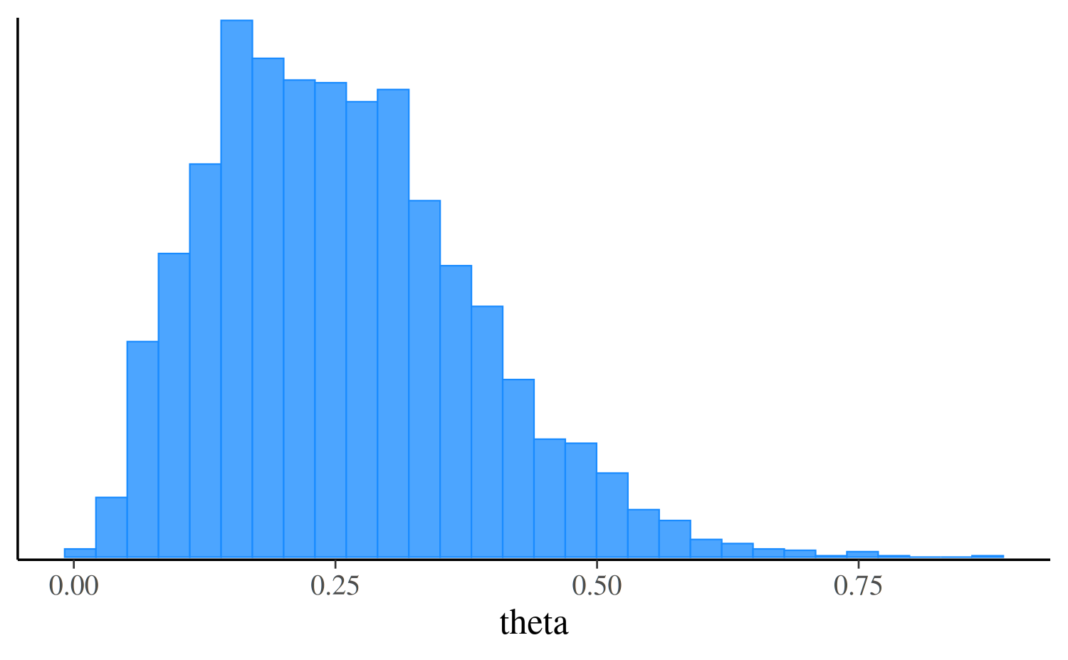
Sampler diagnostics
Extracting diagnostic values for each iteration and chain
The $sampler_diagnostics()
method extracts the values of the sampler parameters
(treedepth__, divergent__, etc.) in formats
supported by the posterior package. The default is as a
3-D array (iteration x chain x variable).
# this is a draws_array object from the posterior package
str(fit$sampler_diagnostics())
'draws_array' num [1:1000, 1:4, 1:6] 0.688 0.811 1 0.966 0.976 ...
- attr(*, "dimnames")=List of 3
..$ iteration: chr [1:1000] "1" "2" "3" "4" ...
..$ chain : chr [1:4] "1" "2" "3" "4"
..$ variable : chr [1:6] "accept_stat__" "stepsize__" "treedepth__" "n_leapfrog__" ...
# this is a draws_df object from the posterior package
str(fit$sampler_diagnostics(format = "df"))
draws_df [4,000 × 9] (S3: draws_df/draws/tbl_df/tbl/data.frame)
$ accept_stat__: num [1:4000] 0.688 0.811 1 0.966 0.976 ...
$ stepsize__ : num [1:4000] 0.905 0.905 0.905 0.905 0.905 ...
$ treedepth__ : num [1:4000] 2 1 2 2 2 1 2 1 2 1 ...
$ n_leapfrog__ : num [1:4000] 3 3 3 3 3 3 3 3 3 3 ...
$ divergent__ : num [1:4000] 0 0 0 0 0 0 0 0 0 0 ...
$ energy__ : num [1:4000] 8.95 8.77 7.87 7.64 6.93 ...
$ .chain : int [1:4000] 1 1 1 1 1 1 1 1 1 1 ...
$ .iteration : int [1:4000] 1 2 3 4 5 6 7 8 9 10 ...
$ .draw : int [1:4000] 1 2 3 4 5 6 7 8 9 10 ...Sampler diagnostic warnings and summaries
The $diagnostic_summary() method will display any
sampler diagnostic warnings and return a summary of diagnostics for each
chain.
fit$diagnostic_summary()$num_divergent
[1] 0 0 0 0
$num_max_treedepth
[1] 0 0 0 0
$ebfmi
[1] 1.114870 1.030279 1.053383 1.077471We see the number of divergences for each of the four chains, the number of times the maximum treedepth was hit for each chain, and the E-BFMI for each chain.
In this case there were no warnings, so in order to demonstrate the warning messages we’ll use one of the CmdStanR example models that suffers from divergences.
fit_with_warning <- cmdstanr_example("schools")Warning: 119 of 4000 (3.0%) transitions ended with a divergence.
See https://mc-stan.org/misc/warnings for details.Warning: 1 of 4 chains had an E-BFMI less than 0.3.
See https://mc-stan.org/misc/warnings for details.After fitting there is a warning about divergences. We can also
regenerate this warning message later using
fit_with_warning$diagnostic_summary().
diagnostics <- fit_with_warning$diagnostic_summary()Warning: 119 of 4000 (3.0%) transitions ended with a divergence.
See https://mc-stan.org/misc/warnings for details.Warning: 1 of 4 chains had an E-BFMI less than 0.3.
See https://mc-stan.org/misc/warnings for details.
print(diagnostics)$num_divergent
[1] 3 54 20 42
$num_max_treedepth
[1] 0 0 0 0
$ebfmi
[1] 0.2709927 0.3625987 0.3117667 0.3331180
# number of divergences reported in warning is the sum of the per chain values
sum(diagnostics$num_divergent)
[1] 119Running optimization and variational inference
CmdStanR also supports running Stan’s optimization algorithms and its
algorithms for variational approximation of full Bayesian inference.
These are run via the $optimize(), $laplace(),
$variational(), and $pathfinder() methods,
which are called in a similar way to the $sample() method
demonstrated above.
Optimization
We can find a mode of the target using $optimize().
The point estimate is extracted with the $mle() method (the
method name is retained for historical reasons).
fit_optim <- mod$optimize(data = data_list, seed = 123)Initial log joint probability = -16.144
Iter log prob ||dx|| ||grad|| alpha alpha0 # evals Notes
6 -5.00402 0.000246518 8.73164e-07 1 1 9
Optimization terminated normally:
Convergence detected: relative gradient magnitude is below tolerance
Finished in 0.1 seconds.
fit_optim$print() # includes lp__ (log prob calculated by Stan program) variable estimate
lp__ -5.00
theta 0.20
fit_optim$mle("theta") theta
0.2000001 Here’s a plot comparing the optimized point estimate to the posterior
of theta.
Warning: Using `size` aesthetic for lines was deprecated in ggplot2 3.4.0.
ℹ Please use `linewidth` instead.
ℹ The deprecated feature was likely used in the bayesplot package.
  Please report the issue at <https://github.com/stan-dev/bayesplot/issues/>.
This warning is displayed once per session.
Call `lifecycle::last_lifecycle_warnings()` to see where this warning was
generated.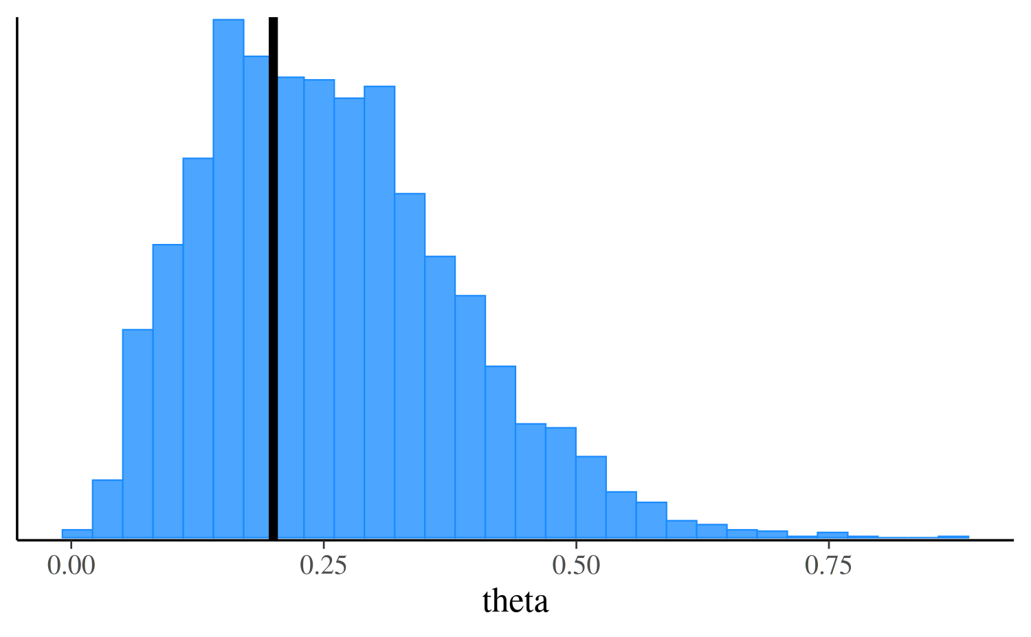
For optimization, by default the mode is calculated without the
Jacobian adjustment for constrained variables, which finds a mode of the
target in the constrained parameter space, whereas
jacobian = TRUE finds a mode of the corresponding density
in the unconstrained space. See the Jacobian
adjustments section of the CmdStan User’s Guide for more
details.
fit_optim_jacobian <- mod$optimize(
  data = data_list,
  jacobian = TRUE,
  seed = 123
)
Initial log joint probability = -18.2733
Iter log prob ||dx|| ||grad|| alpha alpha0 # evals Notes
5 -6.74802 0.000708195 1.43227e-05 1 1 8
Optimization terminated normally:
Convergence detected: relative gradient magnitude is below tolerance
Finished in 0.1 seconds.Laplace Approximation
The $laplace()
method produces a sample from a normal approximation centered at the
mode of a distribution in the unconstrained space. When the mode was
found with the Jacobian adjustment, the draws provide an estimate of the
mean and standard deviation of the posterior distribution. The Laplace
jacobian setting must match the setting used for
optimization so that both use the same target density. See the Laplace
Sampling chapter of the CmdStan User’s Guide for more details.
Here we pass in the fit_optim_jacobian object from above
as the mode argument. If mode is omitted then
optimization will be run internally before taking draws from the normal
approximation.
fit_laplace <- mod$laplace(
    mode = fit_optim_jacobian,
    draws = 4000,
    data = data_list,
    seed = 123,
    refresh = 1000
  )
Calculating Hessian
Calculating inverse of Cholesky factor
Generating draws
iteration: 0
iteration: 1000
iteration: 2000
iteration: 3000
Finished in 0.1 seconds.
fit_laplace$print("theta") variable mean median sd mad q5 q95
theta 0.27 0.25 0.12 0.12 0.10 0.51
mcmc_hist(fit_laplace$draws("theta"), binwidth = 0.025)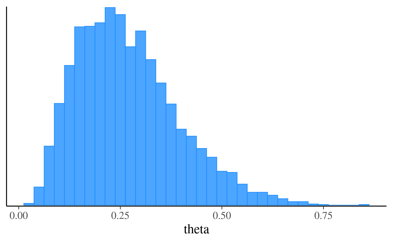
Variational (ADVI)
We can run Stan’s experimental Automatic Differentiation Variational
Inference (ADVI) using the $variational()
method. For details on the ADVI algorithm see the CmdStan
User’s Guide.
fit_vb <- mod$variational(
  data = data_list,
  seed = 123,
  draws = 4000
)
------------------------------------------------------------
EXPERIMENTAL ALGORITHM:
This procedure has not been thoroughly tested and may be unstable
or buggy. The interface is subject to change.
------------------------------------------------------------
Gradient evaluation took 2e-06 seconds
1000 transitions using 10 leapfrog steps per transition would take 0.02 seconds.
Adjust your expectations accordingly!
Begin eta adaptation.
Iteration: 1 / 250 [ 0%] (Adaptation)
Iteration: 50 / 250 [ 20%] (Adaptation)
Iteration: 100 / 250 [ 40%] (Adaptation)
Iteration: 150 / 250 [ 60%] (Adaptation)
Iteration: 200 / 250 [ 80%] (Adaptation)
Success! Found best value [eta = 1] earlier than expected.
Begin stochastic gradient ascent.
iter ELBO delta_ELBO_mean delta_ELBO_med notes
100 -6.164 1.000 1.000
200 -6.225 0.505 1.000
300 -6.186 0.339 0.010 MEDIAN ELBO CONVERGED
Drawing a sample of size 4000 from the approximate posterior...
COMPLETED.
Finished in 0.1 seconds.
fit_vb$print("theta") variable mean median sd mad q5 q95
theta 0.26 0.24 0.11 0.11 0.11 0.46
mcmc_hist(fit_vb$draws("theta"), binwidth = 0.025)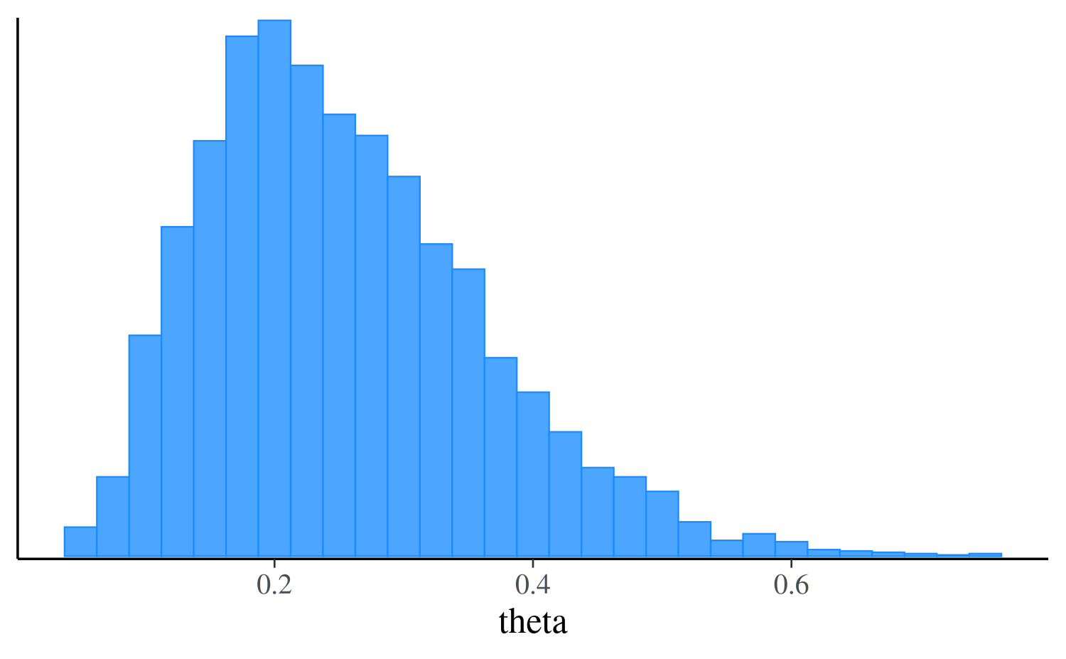
Variational (Pathfinder)
Stan version 2.33 introduced the Pathfinder variational inference
method. For details on how Pathfinder works see the section in the CmdStan
User’s Guide. Pathfinder is run using the $pathfinder()
method.
fit_pf <- mod$pathfinder(
  data = data_list,
  seed = 123,
  draws = 4000
)
Path [1] :Initial log joint density = -18.273334
Path [1] : Iter log prob ||dx|| ||grad|| alpha alpha0 # evals ELBO Best ELBO Notes
5 -6.748e+00 7.082e-04 1.432e-05 1.000e+00 1.000e+00 156 -6.216e+00 -6.145e+00
Path [1] :Best Iter: [5] ELBO (-6.145070) evaluations: (156)
Path [2] :Initial log joint density = -19.192715
Path [2] : Iter log prob ||dx|| ||grad|| alpha alpha0 # evals ELBO Best ELBO Notes
5 -6.748e+00 2.015e-04 2.228e-06 1.000e+00 1.000e+00 156 -6.170e+00 -6.223e+00
Path [2] :Best Iter: [2] ELBO (-6.170358) evaluations: (156)
Path [3] :Initial log joint density = -6.774820
Path [3] : Iter log prob ||dx|| ||grad|| alpha alpha0 # evals ELBO Best ELBO Notes
4 -6.748e+00 1.137e-04 2.596e-07 1.000e+00 1.000e+00 123 -6.243e+00 -6.178e+00
Path [3] :Best Iter: [4] ELBO (-6.177909) evaluations: (123)
Path [4] :Initial log joint density = -7.949193
Path [4] : Iter log prob ||dx|| ||grad|| alpha alpha0 # evals ELBO Best ELBO Notes
5 -6.748e+00 2.145e-04 1.301e-06 1.000e+00 1.000e+00 156 -6.235e+00 -6.197e+00
Path [4] :Best Iter: [5] ELBO (-6.197118) evaluations: (156)
Finished in 0.1 seconds.
fit_pf$print("theta") variable mean median sd mad q5 q95
theta 0.25 0.24 0.12 0.12 0.08 0.47Let’s extract the draws, make the same plot we made after running the other algorithms, and compare them all. In this simple example the distributions are quite similar, but this will not always be the case for more challenging problems.
mcmc_hist(fit_pf$draws("theta"), binwidth = 0.025) +
  ggplot2::labs(subtitle = "Approximate posterior from pathfinder") +
  ggplot2::xlim(0, 1)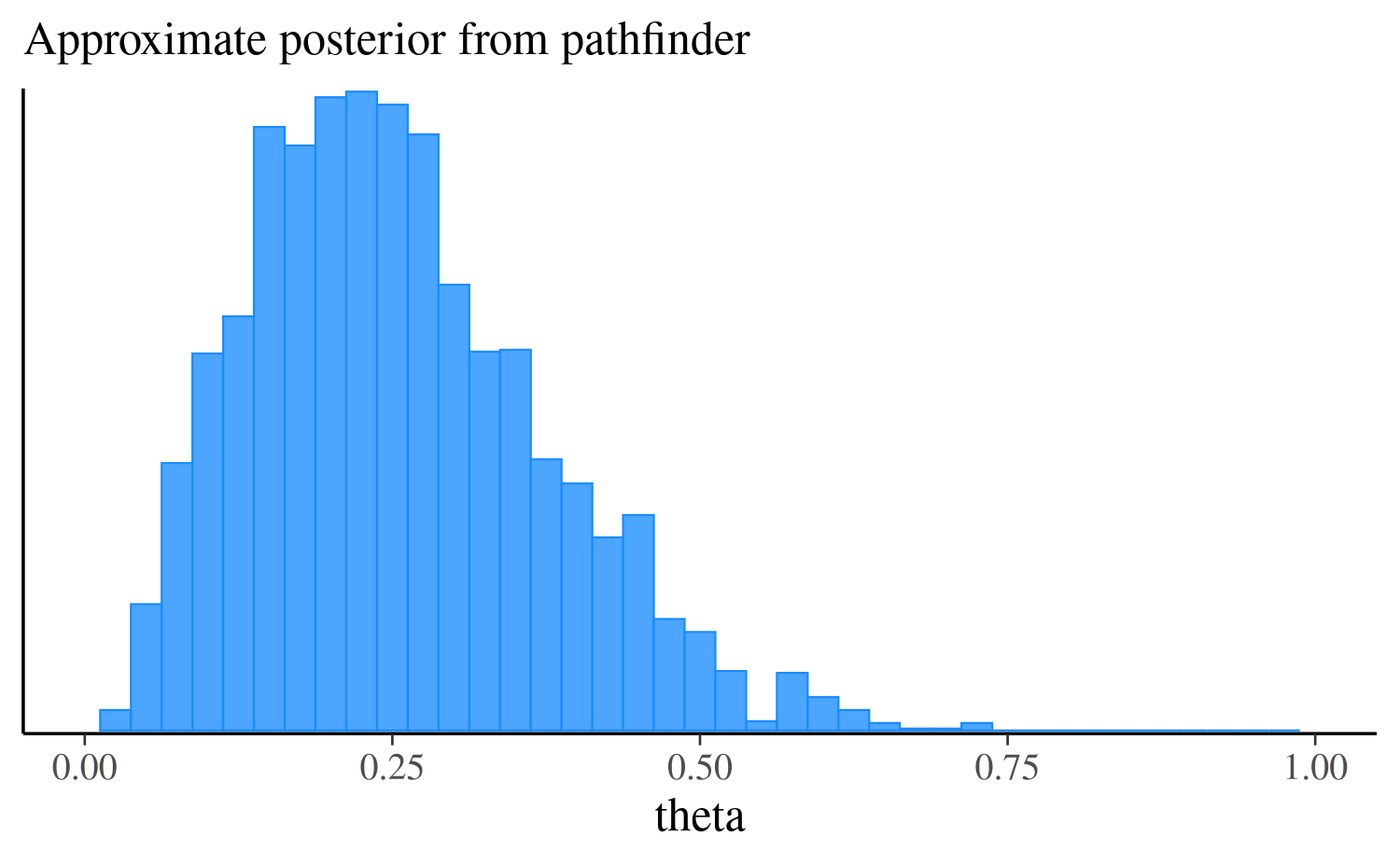
mcmc_hist(fit_vb$draws("theta"), binwidth = 0.025) +
  ggplot2::labs(subtitle = "Approximate posterior from variational") +
  ggplot2::xlim(0, 1)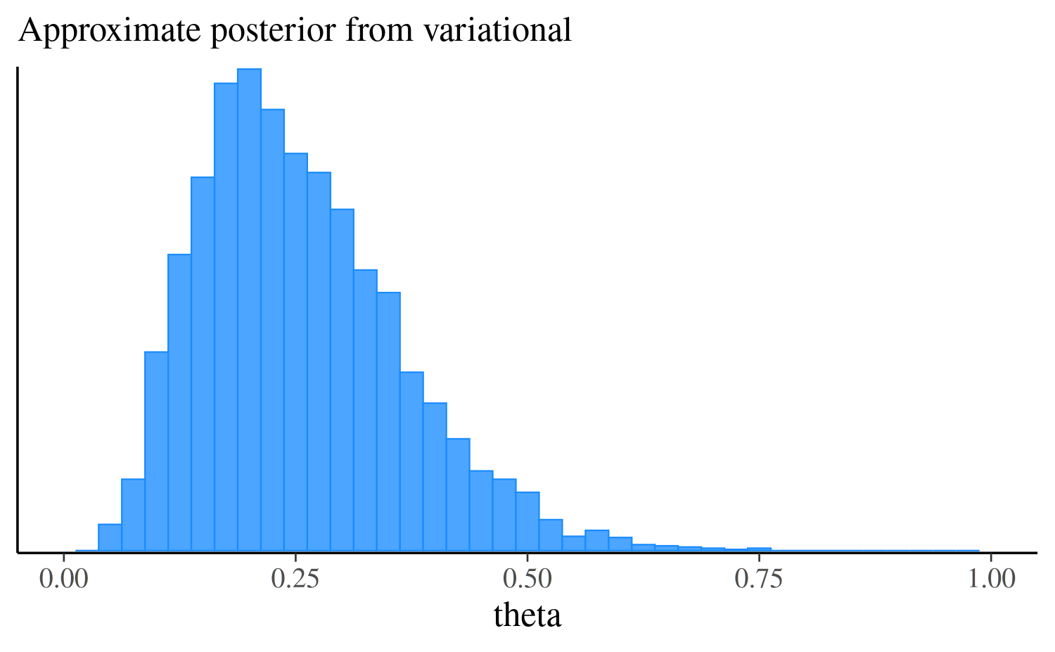
mcmc_hist(fit_laplace$draws("theta"), binwidth = 0.025) +
  ggplot2::labs(subtitle = "Approximate posterior from Laplace") +
  ggplot2::xlim(0, 1)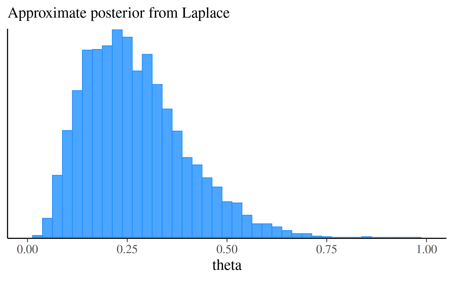
mcmc_hist(fit$draws("theta"), binwidth = 0.025) +
  ggplot2::labs(subtitle = "Posterior from MCMC") +
  ggplot2::xlim(0, 1)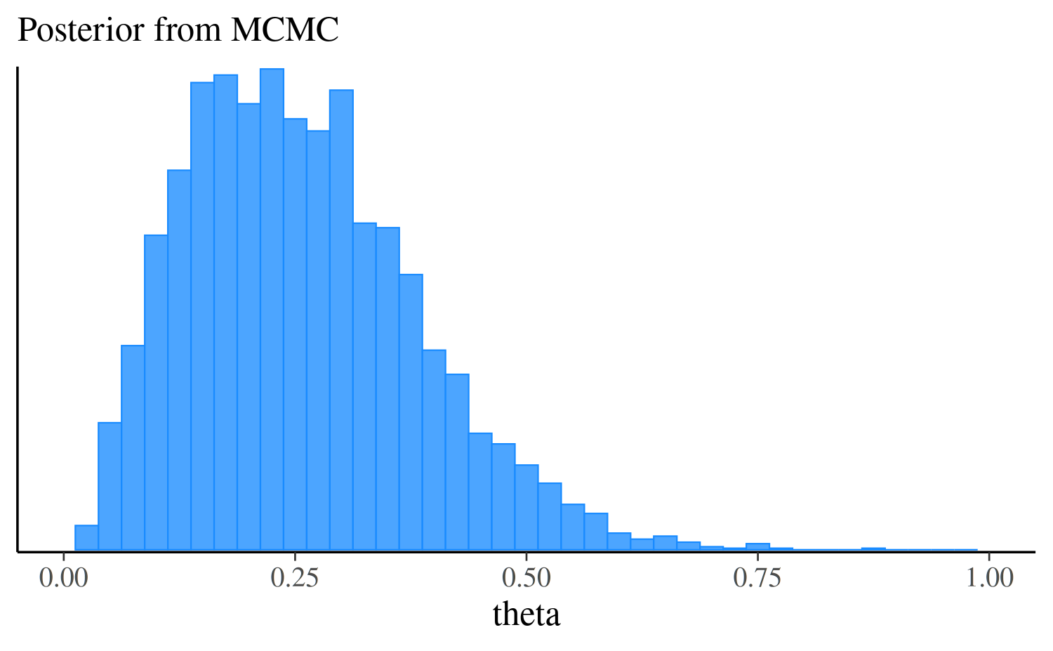
For more details on the $optimize(),
$laplace(), $variational(), and
$pathfinder() methods, follow these links to their
documentation pages.
Running standalone generated quantities
The $generate_quantities()
method runs a Stan program’s generated quantities block
using parameter values from a previous fit, without rerunning inference.
It accepts fitted model objects produced by any of the fitting methods
described above. See the method documentation for details and a complete
example.
Saving fitted model objects
The $save_object()
method provided by CmdStanR is the most convenient way to save a fitted
model object to disk and ensure that all of the contents are available
when reading the object back into R. By default,
fit$save_object() will use the RDS format to
save the object. The saved object can then be read back into R using
readRDS().
fit$save_object(file = "fit.RDS")

fit2 <- readRDS("fit.RDS")
But if your model object is large, then
fit$save_object() can take a long time if saving in the
default RDS format. For large objects, we recommend using the much
faster qs2
format. The saved object can then be read back into R using
qs2::qs_read().
fit$save_object(file = "fit.qs2", format = "qs2")

fit2 <- qs2::qs_read("fit.qs2")
Comparison with RStan
Different ways of interfacing with Stan’s C++
The RStan interface (rstan package)
provides its core functionality through an in-memory interface to Stan
and relies on R packages such as Rcpp to call C++ code
from R. CmdStanR’s core model compilation and inference workflow instead
runs CmdStan in external processes and reads the resulting output files.
Only optional CmdStanR features, such as
$expose_functions() and the additional model methods, use
Rcpp to call compiled C++ code directly from R.
Advantages of RStan
-
CRAN provides binary versions of RStan for Windows and macOS. RStan-based packages can also include precompiled Stan models in their binary packages, which allows users to run the models without a local C++ toolchain.
CmdStanR-based packages can use
instantiateto compile models once during package installation. Because CRAN’s build machines do not provide CmdStan, packages using this workflow currently need to be installed from source with CmdStan and a C++ toolchain available. Avoids use of R6 classes, which may result in more familiar syntax for many R users.
Advantages of CmdStanR
CmdStan is installed separately from CmdStanR, so users can often update to a new Stan release by updating CmdStan without waiting for a new CmdStanR release.
Running CmdStan in external processes isolates inference from the R process, reducing the risk that a failure during inference terminates the R session.
Potentially lower memory use in the R session. CmdStan writes results to CSV files, and CmdStanR loads draws into R only when requested. This can avoid retaining all output in memory during fitting.
More permissive license. RStan uses the GPL (>= 3) license while the license for CmdStanR is BSD 3-clause, which is a bit more permissive and is the same license used for CmdStan and the Stan C++ source code.
Additional resources
There are additional vignettes available that discuss many other aspects of using CmdStanR. These can be found online at the CmdStanR website:
To ask a question please post on the Stan forums:
To report a bug, suggest a feature (including additions to these vignettes), or to start contributing to CmdStanR development (new contributors welcome!) please open an issue on GitHub: