Run Stan's Laplace algorithm

The $laplace() method of a CmdStanModel object produces a sample from a normal approximation centered at the mode of a distribution in the unconstrained space. If the mode is a maximum a posteriori (MAP) estimate, the samples provide an estimate of the mean and standard deviation of the posterior distribution. If the mode is a maximum likelihood estimate (MLE), the sample provides an estimate of the standard error of the likelihood. Whether the mode is the MAP or MLE depends on the value of the jacobian argument when running optimization. See the CmdStan User’s Guide for more details.

Any argument left as NULL will default to the default value used by the installed version of CmdStan.

laplace(
  data = NULL,
  seed = NULL,
  refresh = NULL,
  init = NULL,
  save_latent_dynamics = FALSE,
  output_dir = getOption("cmdstanr_output_dir"),
  output_basename = NULL,
  sig_figs = NULL,
  threads = NULL,
  opencl_ids = NULL,
  mode = NULL,
  opt_args = NULL,
  jacobian = TRUE,
  draws = NULL,
  show_messages = TRUE,
  show_exceptions = TRUE,
  save_cmdstan_config = NULL
)

Arguments

data

(multiple options) The data to use for the variables specified in the data block of the Stan program. One of the following:

A named list of R objects with the names corresponding to variables declared in the data block of the Stan program. Internally this list is then written to JSON for CmdStan using write_stan_json(). See write_stan_json() for details on the conversions performed on R objects before they are passed to Stan.
A path to a data file compatible with CmdStan (JSON or R dump). See the appendices in the CmdStan guide for details on using these formats.
NULL or an empty list if the Stan program has no data block.

seed

(positive integer(s)) A seed for the (P)RNG to pass to CmdStan. In the case of multi-chain sampling the single seed will automatically be augmented by the the run (chain) ID so that each chain uses a different seed. The exception is the transformed data block, which defaults to using same seed for all chains so that the same data is generated for all chains if RNG functions are used. The only time seed should be specified as a vector (one element per chain) is if RNG functions are used in transformed data and the goal is to generate different data for each chain.

refresh

(non-negative integer) The number of iterations between printed screen updates. If refresh = 0, only error messages will be printed.

init

(multiple options) The initialization method to use for the variables declared in the parameters block of the Stan program. One of the following:

A real number x>0. This initializes all parameters randomly between [-x,x] on the unconstrained parameter space.;
The number 0. This initializes all parameters to 0;
A character vector of paths (one per chain) to JSON or Rdump files containing initial values for all or some parameters. See write_stan_json() to write R objects to JSON files compatible with CmdStan.
A list of lists containing initial values for all or some parameters. For MCMC the list should contain a sublist for each chain. For other model fitting methods there should be just one sublist. The sublists should have named elements corresponding to the parameters for which you are specifying initial values. See Examples.
A function that returns a single list with names corresponding to the parameters for which you are specifying initial values. The function can take no arguments or a single argument chain_id. For MCMC, if the function has argument chain_id it will be supplied with the chain id (from 1 to number of chains) when called to generate the initial values. See Examples.
A CmdStanMCMC, CmdStanMLE, CmdStanVB, CmdStanPathfinder, or CmdStanLaplace fit object. If the fit object's parameters are only a subset of the model parameters then the other parameters will be drawn by Stan's default initialization. The fit object must have at least some parameters that are the same name and dimensions as the current Stan model. For the sample and pathfinder method, if the fit object has fewer draws than the requested number of chains/paths then the inits will be drawn using sampling with replacement. Otherwise sampling without replacement will be used. When a CmdStanPathfinder fit object is used as the init, if . psis_resample was set to FALSE and calculate_lp was set to TRUE (default), then resampling without replacement with Pareto smoothed weights will be used. If psis_resample was set to TRUE or calculate_lp was set to FALSE then sampling without replacement with uniform weights will be used to select the draws. PSIS resampling is used to select the draws for CmdStanVB, and CmdStanLaplace fit objects.
A type inheriting from posterior::draws. If the draws object has less samples than the number of requested chains/paths then the inits will be drawn using sampling with replacement. Otherwise sampling without replacement will be used. If the draws object's parameters are only a subset of the model parameters then the other parameters will be drawn by Stan's default initialization. The fit object must have at least some parameters that are the same name and dimensions as the current Stan model.

save_latent_dynamics

Ignored for this method.

output_dir

(string) A path to a directory where CmdStan should write its output CSV files. For MCMC there will be one file per chain; for other methods there will be a single file. For interactive use this can typically be left at NULL (temporary directory) since CmdStanR makes the CmdStan output (posterior draws and diagnostics) available in R via methods of the fitted model objects. This can be set for an entire R session using options(cmdstanr_output_dir). The behavior of output_dir is as follows:

If NULL (the default), then the CSV files are written to a temporary directory and only saved permanently if the user calls one of the $save_* methods of the fitted model object (e.g., $save_output_files()). These temporary files are removed when the fitted model object is garbage collected (manually or automatically).
If a path, then the files are created in output_dir with names corresponding to the defaults used by $save_output_files().

output_basename

(string) A string to use as a prefix for the names of the output CSV files of CmdStan. If NULL (the default), the basename of the output CSV files will be comprised from the model name, timestamp, and 5 random characters.

sig_figs

(positive integer) The number of significant figures used when storing the output values. By default, CmdStan represent the output values with 6 significant figures. The upper limit for sig_figs is 18. Increasing this value will result in larger output CSV files and thus an increased usage of disk space.

threads

(positive integer) If the model was compiled with threading support, the number of threads to use in parallelized sections (e.g., when using the Stan functions reduce_sum() or map_rect()).

opencl_ids

(integer vector of length 2) The platform and device IDs of the OpenCL device to use for fitting. The model must be compiled with cpp_options = list(stan_opencl = TRUE) for this argument to have an effect.

mode

(multiple options) The mode to center the approximation at. One of the following:

A CmdStanMLE object from a previous run of $optimize().
The path to a CmdStan CSV file from running optimization.
NULL, in which case $optimize() will be run with jacobian=jacobian (see the jacobian argument below).

In all cases the total time reported by $time() will be the time of the Laplace sampling step only and does not include the time taken to run the $optimize() method.

opt_args

(named list) A named list of optional arguments to pass to $optimize() if mode=NULL.

jacobian

(logical) Whether or not to enable the Jacobian adjustment for constrained parameters. The default is TRUE. See the Laplace Sampling section of the CmdStan User's Guide for more details. If mode is not NULL then the value of jacobian must match the value used when optimization was originally run. If mode is NULL then the value of jacobian specified here is used when running optimization.

draws

(positive integer) The number of draws to take.

show_messages

(logical) When TRUE (the default), prints all output during the execution process, such as iteration numbers and elapsed times. If the output is silenced then the $output() method of the resulting fit object can be used to display the silenced messages.

show_exceptions

(logical) When TRUE (the default), prints all informational messages, for example rejection of the current proposal. Disable if you wish to silence these messages, but this is not usually recommended unless you are very confident that the model is correct up to numerical error. If the messages are silenced then the $output() method of the resulting fit object can be used to display the silenced messages.

save_cmdstan_config

(logical) When TRUE (the default), call CmdStan with argument "output save_config=1" to save a json file which contains the argument tree and extra information (equivalent to the output CSV file header). This option is only available in CmdStan 2.34.0 and later.

Value

A CmdStanLaplace object.

Examples

# \dontrun{
file <- file.path(cmdstan_path(), "examples/bernoulli/bernoulli.stan")
mod <- cmdstan_model(file)
mod$print()
#> data {
#>   int<lower=0> N;
#>   array[N] int<lower=0, upper=1> y;
#> }
#> parameters {
#>   real<lower=0, upper=1> theta;
#> }
#> model {
#>   theta ~ beta(1, 1); // uniform prior on interval 0,1
#>   y ~ bernoulli(theta);
#> }

stan_data <- list(N = 10, y = c(0,1,0,0,0,0,0,0,0,1))
fit_mode <- mod$optimize(data = stan_data, jacobian = TRUE)
#> Initial log joint probability = -7.3571 
#>     Iter      log prob        ||dx||      ||grad||       alpha      alpha0  # evals  Notes  
#>        5      -6.74802   0.000511122   9.02231e-07           1           1        8    
#> Optimization terminated normally:  
#>   Convergence detected: relative gradient magnitude is below tolerance 
#> Finished in  0.3 seconds.
fit_laplace <- mod$laplace(data = stan_data, mode = fit_mode)
#> Calculating Hessian 
#> Calculating inverse of Cholesky factor 
#> Generating draws 
#> iteration: 0 
#> iteration: 100 
#> iteration: 200 
#> iteration: 300 
#> iteration: 400 
#> iteration: 500 
#> iteration: 600 
#> iteration: 700 
#> iteration: 800 
#> iteration: 900 
#> Finished in  0.2 seconds.
fit_laplace$summary()
#> # A tibble: 3 × 7
#>   variable      mean median    sd   mad     q5      q95
#>   <chr>        <dbl>  <dbl> <dbl> <dbl>  <dbl>    <dbl>
#> 1 lp__        -7.24  -6.97  0.734 0.309 -8.50  -6.75   
#> 2 lp_approx__ -0.491 -0.223 0.698 0.309 -1.80  -0.00200
#> 3 theta        0.271  0.250 0.123 0.123  0.103  0.487  

# if mode isn't specified optimize is run internally first
fit_laplace <- mod$laplace(data = stan_data)
#> Initial log joint probability = -11.0359 
#>     Iter      log prob        ||dx||      ||grad||       alpha      alpha0  # evals  Notes  
#>        5      -6.74802   0.000945646   1.40836e-05           1           1        8    
#> Optimization terminated normally:  
#>   Convergence detected: relative gradient magnitude is below tolerance 
#> Finished in  0.1 seconds.
#> Calculating Hessian 
#> Calculating inverse of Cholesky factor 
#> Generating draws 
#> iteration: 0 
#> iteration: 100 
#> iteration: 200 
#> iteration: 300 
#> iteration: 400 
#> iteration: 500 
#> iteration: 600 
#> iteration: 700 
#> iteration: 800 
#> iteration: 900 
#> Finished in  0.1 seconds.
fit_laplace$summary()
#> # A tibble: 3 × 7
#>   variable      mean median    sd   mad     q5      q95
#>   <chr>        <dbl>  <dbl> <dbl> <dbl>  <dbl>    <dbl>
#> 1 lp__        -7.26  -6.97  0.744 0.306 -8.73  -6.75   
#> 2 lp_approx__ -0.516 -0.226 0.742 0.306 -1.93  -0.00178
#> 3 theta        0.270  0.250 0.126 0.121  0.103  0.513  

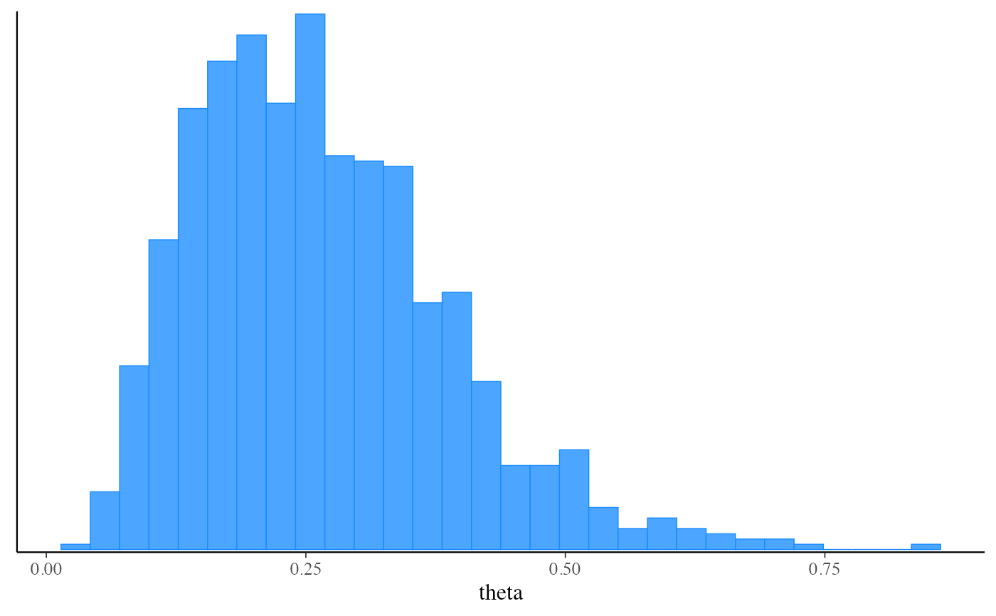
# plot approximate posterior
bayesplot::mcmc_hist(fit_laplace$draws("theta"))
#> `stat_bin()` using `bins = 30`. Pick better value with `binwidth`.

# }

Arguments

Value

See also

Examples