Estimating Generalized Linear Models for Count Data with rstanarm
Jonah Gabry and Ben Goodrich
2025-12-30
Source:vignettes/count.Rmd
count.RmdIntroduction
This vignette explains how to estimate generalized linear models
(GLMs) for count data using the stan_glm function in the
rstanarm package.
The four steps of a Bayesian analysis are
- Specify a joint distribution for the outcome(s) and all the unknowns, which typically takes the form of a marginal prior distribution for the unknowns multiplied by a likelihood for the outcome(s) conditional on the unknowns. This joint distribution is proportional to a posterior distribution of the unknowns conditional on the observed data
- Draw from posterior distribution using Markov Chain Monte Carlo (MCMC).
- Evaluate how well the model fits the data and possibly revise the model.
- Draw from the posterior predictive distribution of the outcome(s) given interesting values of the predictors in order to visualize how a manipulation of a predictor affects (a function of) the outcome(s).
Steps 3 and 4 are covered in more depth by the vignette entitled “How to Use the rstanarm
Package”. This vignette focuses on Step 1 for Poisson and negative
binomial regression models using the stan_glm function.
Likelihood
If the outcome for a single observation \(y\) is assumed to follow a Poisson distribution, the likelihood for one observation can be written as a conditionally Poisson PMF
\[\tfrac{1}{y!} \lambda^y e^{-\lambda},\]
where \(\lambda = E(y | \mathbf{x}) = g^{-1}(\eta)\) and \(\eta = \alpha + \mathbf{x}^\top \boldsymbol{\beta}\) is a linear predictor. For the Poisson distribution it is also true that \(\lambda = Var(y | \mathbf{x})\), i.e. the mean and variance are both \(\lambda\). Later in this vignette we also show how to estimate a negative binomial regression, which relaxes this assumption of equal conditional mean and variance of \(y\).
Because the rate parameter \(\lambda\) must be positive, for a Poisson GLM the link function \(g\) maps between the positive real numbers \(\mathbb{R}^+\) (the support of \(\lambda\)) and the set of all real numbers \(\mathbb{R}\). When applied to a linear predictor \(\eta\) with values in \(\mathbb{R}\), the inverse link function \(g^{-1}(\eta)\) therefore returns a positive real number.
Although other link functions are possible, the canonical link function for a Poisson GLM is the log link \(g(x) = \ln{(x)}\). With the log link, the inverse link function is simply the exponential function and the likelihood for a single observation becomes
\[\frac{g^{-1}(\eta)^y}{y!} e^{-g^{-1}(\eta)} = \frac{e^{\eta y}}{y!} e^{-e^\eta}.\]
Priors
A full Bayesian analysis requires specifying prior distributions
\(f(\alpha)\) and \(f(\boldsymbol{\beta})\) for the intercept
and vector of regression coefficients. When using stan_glm,
these distributions can be set using the prior_intercept
and prior arguments. The stan_glm function
supports a variety of prior distributions, which are explained in the
rstanarm documentation
(help(priors, package = 'rstanarm')).
As an example, suppose we have \(K\)
predictors and believe — prior to seeing the data — that \(\alpha, \beta_1, \dots, \beta_K\) are as
likely to be positive as they are to be negative, but are highly
unlikely to be far from zero. These beliefs can be represented by normal
distributions with mean zero and a small scale (standard deviation). To
give \(\alpha\) and each of the \(\beta\)s this prior (with a scale of 1,
say), in the call to stan_glm we would include the
arguments prior_intercept = normal(0,1) and
prior = normal(0,1).
If, on the other hand, we have less a priori confidence that the parameters will be close to zero then we could use a larger scale for the normal distribution and/or a distribution with heavier tails than the normal like the Student t distribution. Step 1 in the “How to Use the rstanarm Package” vignette discusses one such example.
Posterior
With independent prior distributions, the joint posterior distribution for \(\alpha\) and \(\boldsymbol{\beta}\) in the Poisson model is proportional to the product of the priors and the \(N\) likelihood contributions:
\[f\left(\alpha,\boldsymbol{\beta} | \mathbf{y},\mathbf{X}\right) \propto f\left(\alpha\right) \times \prod_{k=1}^K f\left(\beta_k\right) \times \prod_{i=1}^N { \frac{g^{-1}(\eta_i)^{y_i}}{y_i!} e^{-g^{-1}(\eta_i)}}.\]
This is posterior distribution that stan_glm will draw
from when using MCMC.
Poisson and Negative Binomial Regression Example
This example comes from Chapter 8.3 of Gelman and Hill (2007).
We want to make inferences about the efficacy of a certain pest management system at reducing the number of roaches in urban apartments. Here is how Gelman and Hill describe the experiment (pg. 161):
[…] the treatment and control were applied to 160 and 104 apartments, respectively, and the outcome measurement \(y_i\) in each apartment \(i\) was the number of roaches caught in a set of traps. Different apartments had traps for different numbers of days […]
In addition to an intercept, the regression predictors for the model
are the pre-treatment number of roaches roach1, the
treatment indicator treatment, and a variable indicating
whether the apartment is in a building restricted to elderly residents
senior. Because the number of days for which the roach
traps were used is not the same for all apartments in the sample, we
include it as an exposure, which slightly changes the model described in
the Likelihood section above in that the rate parameter
\(\lambda_i =
exp(\eta_i)\) is multiplied by the exposure \(u_i\) giving us \(y_i \sim Poisson(u_i \lambda_i)\). This is
equivalent to adding \(\ln{(u_i)}\) to
the linear predictor \(\eta_i\) and it
can be specified using the offset argument to
stan_glm.
library(rstanarm)
data(roaches)

# Rescale
roaches$roach1 <- roaches$roach1 / 100
# Estimate original model
glm1 <- glm(y ~ roach1 + treatment + senior, offset = log(exposure2),
            data = roaches, family = poisson)
# Estimate Bayesian version with stan_glm
stan_glm1 <- stan_glm(y ~ roach1 + treatment + senior, offset = log(exposure2),
                      data = roaches, family = poisson,
                      prior = normal(0, 2.5),
                      prior_intercept = normal(0, 5),
                      seed = 12345)
The formula, data, family, and
offset arguments to stan_glm can be specified
in exactly the same way as for glm. The
poisson family function defaults to using the log link, but
to write code readable to someone not familiar with the defaults we
should be explicit and use
family = poisson(link = "log").
We’ve also specified some optional arguments. The chains
argument controls how many Markov chains are executed, the
cores argument controls the number of cores utilized by the
computer when fitting the model. We also provided a seed so that we have
the option to deterministically reproduce these results at any time. The
stan_glm function has many other optional arguments that
allow for more user control over the way estimation is performed. The
documentation for stan_glm has more information about these
controls as well as other topics related to GLM estimation.
Here are the point estimates and uncertainties from the
glm fit and stan_glm fit, which we see are
nearly identical:
         (Intercept) roach1 treatment senior
glm             3.09    0.7     -0.52  -0.38
stan_glm        3.09    0.7     -0.52  -0.38
round(rbind(glm = summary(glm1)$coefficients[, "Std. Error"],
            stan_glm = se(stan_glm1)), digits = 3)
(Intercept) roach1 treatment senior
glm 0.021 0.009 0.025 0.033
stan_glm 0.021 0.009 0.024 0.034(Note: the dataset we have is slightly different from the one used in
Gelman and Hill (2007), which leads to slightly different parameter
estimates than those shown in the book even when copying the
glm call verbatim. Also, we have rescaled the
roach1 predictor. For the purposes of this example, the
actual estimates are less important than the process.)
Gelman and Hill next show how to compare the observed data to
replicated datasets from the model to check the quality of the fit. Here
we don’t show the original code used by Gelman and Hill because it’s
many lines, requiring several loops and some care to get the matrix
multiplications right (see pg. 161-162). On the other hand, the
rstanarm package makes this easy. We can generate
replicated datasets with a single line of code using the
posterior_predict function:
yrep <- posterior_predict(stan_glm1)By default posterior_predict will generate a dataset for
each set of parameter draws from the posterior distribution. That is,
yrep will be an \(S \times
N\) matrix, where \(S\) is the
size of the posterior sample and \(N\)
is the number of data points. Each row of yrep represents a
full dataset generated from the posterior predictive distribution. For
more about the importance of the posterior_predict
function, see the “How to Use the
rstanarm Package” vignette.
Gelman and Hill take the simulated datasets and for each of them
compute the proportion of zeros and compare to the observed proportion
in the original data. We can do this easily using the
pp_check function, which generates graphical comparisons of
the data y and replicated datasets yrep.
prop_zero <- function(y) mean(y == 0)
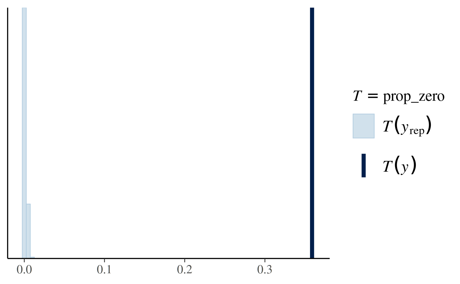
(prop_zero_test1 <- pp_check(stan_glm1, plotfun = "stat", stat = "prop_zero", binwidth = .005))
The value of the test statistic (in this case the proportion of
zeros) computed from the sample y is the dark blue vertical
line. More than 30% of these observations are zeros, whereas the
replicated datasets all contain less than 1% zeros (light blue
histogram). This is a sign that we should consider a model that more
accurately accounts for the large proportion of zeros in the data.
Gelman and Hill show how we can do this using an overdispersed Poisson
regression. To illustrate the use of a different stan_glm
model, here we will instead try negative
binomial regression, which is also used for overdispersed or
zero-inflated count data. The negative binomial distribution allows the
(conditional) mean and variance of \(y\) to differ unlike the Poisson
distribution. To fit the negative binomial model can either use the
stan_glm.nb function or, equivalently, change the
family we specify in the call to stan_glm to
neg_binomial_2 instead of poisson. To do the
latter we can just use update:
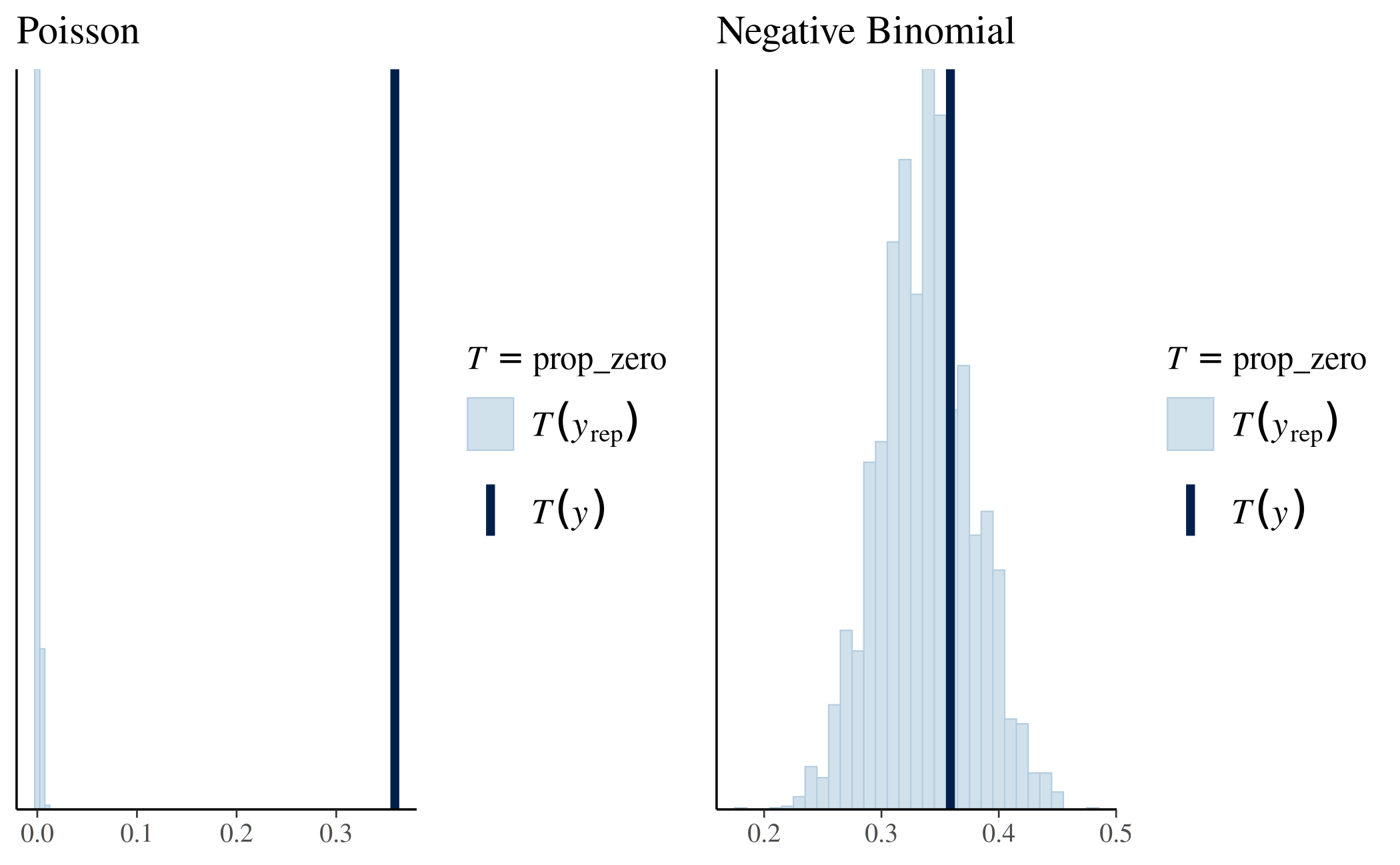
stan_glm2 <- update(stan_glm1, family = neg_binomial_2) We now use pp_check again, this time to check the
proportion of zeros in the replicated datasets under the negative
binomial model:
prop_zero_test2 <- pp_check(stan_glm2, plotfun = "stat", stat = "prop_zero",
                            binwidth = 0.01)
# Show graphs for Poisson and negative binomial side by side
bayesplot_grid(prop_zero_test1 + ggtitle("Poisson"),
               prop_zero_test2 + ggtitle("Negative Binomial"),
               grid_args = list(ncol = 2))
This is a much better fit, as the proportion of zeros in the data falls nicely near the center of the distribution of the proportion of zeros among the replicated datasets. The observed proportion of zeros is quite plausible under this model.
We could have also made these plots manually without using the
pp_check function because we have the yrep
datasets created by posterior_predict. The
pp_check function takes care of this for us, but
yrep can be used directly to carry out other posterior
predictive checks that aren’t automated by pp_check.
When we comparing the models using the loo package we also see a clear preference for the negative binomial model
loo1 <- loo(stan_glm1, cores = 1)
loo2 <- loo(stan_glm2, cores = 1)
loo_compare(loo1, loo2)
elpd_diff se_diff
stan_glm2 0.0 0.0
stan_glm1 -5345.4 706.7which is not surprising given the better fit we’ve already observed from the posterior predictive checks.