Bayesian generalized linear models via Stan

Generalized linear modeling with optional prior distributions for the coefficients, intercept, and auxiliary parameters.

Usage

stan_glm(
  formula,
  family = gaussian(),
  data,
  weights,
  subset,
  na.action = NULL,
  offset = NULL,
  model = TRUE,
  x = FALSE,
  y = TRUE,
  contrasts = NULL,
  ...,
  prior = default_prior_coef(family),
  prior_intercept = default_prior_intercept(family),
  prior_aux = exponential(autoscale = TRUE),
  prior_PD = FALSE,
  algorithm = c("sampling", "optimizing", "meanfield", "fullrank"),
  mean_PPD = algorithm != "optimizing" && !prior_PD,
  adapt_delta = NULL,
  QR = FALSE,
  sparse = FALSE
)

stan_glm.nb(
  formula,
  data,
  weights,
  subset,
  na.action = NULL,
  offset = NULL,
  model = TRUE,
  x = FALSE,
  y = TRUE,
  contrasts = NULL,
  link = "log",
  ...,
  prior = default_prior_coef(family),
  prior_intercept = default_prior_intercept(family),
  prior_aux = exponential(autoscale = TRUE),
  prior_PD = FALSE,
  algorithm = c("sampling", "optimizing", "meanfield", "fullrank"),
  mean_PPD = algorithm != "optimizing",
  adapt_delta = NULL,
  QR = FALSE
)

stan_glm.fit(
  x,
  y,
  weights = rep(1, NROW(y)),
  offset = rep(0, NROW(y)),
  family = gaussian(),
  ...,
  prior = default_prior_coef(family),
  prior_intercept = default_prior_intercept(family),
  prior_aux = exponential(autoscale = TRUE),
  prior_smooth = exponential(autoscale = FALSE),
  prior_ops = NULL,
  group = list(),
  prior_PD = FALSE,
  algorithm = c("sampling", "optimizing", "meanfield", "fullrank"),
  mean_PPD = algorithm != "optimizing" && !prior_PD,
  adapt_delta = NULL,
  QR = FALSE,
  sparse = FALSE,
  importance_resampling = algorithm != "sampling",
  keep_every = algorithm != "sampling"
)

Arguments

formula, data, subset

Same as glm, but we strongly advise against omitting the data argument. Unless data is specified (and is a data frame) many post-estimation functions (including update, loo, kfold) are not guaranteed to work properly.

family

Same as glm, except negative binomial GLMs are also possible using the neg_binomial_2 family object.

na.action, contrasts

Same as glm, but rarely specified.

model, offset, weights

Same as glm.

x

In stan_glm, logical scalar indicating whether to return the design matrix. In stan_glm.fit, usually a design matrix but can also be a list of design matrices with the same number of rows, in which case the first element of the list is interpreted as the primary design matrix and the remaining list elements collectively constitute a basis for a smooth nonlinear function of the predictors indicated by the formula argument to stan_gamm4.

y

In stan_glm, logical scalar indicating whether to return the response vector. In stan_glm.fit, a response vector.

...

Further arguments passed to the function in the rstan package (sampling, vb, or optimizing), corresponding to the estimation method named by algorithm. For example, if algorithm is "sampling" it is possible to specify iter, chains, cores, and other MCMC controls.

Another useful argument that can be passed to rstan via ... is refresh, which specifies how often to print updates when sampling (i.e., show the progress every refresh iterations). refresh=0 turns off the iteration updates.

prior

The prior distribution for the (non-hierarchical) regression coefficients.

The default priors are described in the vignette Prior Distributions for rstanarm Models. If not using the default, prior should be a call to one of the various functions provided by rstanarm for specifying priors. The subset of these functions that can be used for the prior on the coefficients can be grouped into several "families":

Family	Functions
Student t family	normal, student_t, cauchy
Hierarchical shrinkage family	hs, hs_plus
Laplace family	laplace, lasso
Product normal family	product_normal

See the priors help page for details on the families and how to specify the arguments for all of the functions in the table above. To omit a prior —i.e., to use a flat (improper) uniform prior— prior can be set to NULL, although this is rarely a good idea.

Note: Unless QR=TRUE, if prior is from the Student t family or Laplace family, and if the autoscale argument to the function used to specify the prior (e.g. normal) is left at its default and recommended value of TRUE, then the default or user-specified prior scale(s) may be adjusted internally based on the scales of the predictors. See the priors help page and the Prior Distributions vignette for details on the rescaling and the prior_summary function for a summary of the priors used for a particular model.

prior_intercept

The prior distribution for the intercept (after centering all predictors, see note below).

The default prior is described in the vignette Prior Distributions for rstanarm Models. If not using the default, prior_intercept can be a call to normal, student_t or cauchy. See the priors help page for details on these functions. To omit a prior on the intercept —i.e., to use a flat (improper) uniform prior— prior_intercept can be set to NULL.

Note: If using a dense representation of the design matrix —i.e., if the sparse argument is left at its default value of FALSE— then the prior distribution for the intercept is set so it applies to the value when all predictors are centered (you don't need to manually center them). This is explained further in [Prior Distributions for rstanarm Models](https://mc-stan.org/rstanarm/articles/priors.html) If you prefer to specify a prior on the intercept without the predictors being auto-centered, then you have to omit the intercept from the formula and include a column of ones as a predictor, in which case some element of prior specifies the prior on it, rather than prior_intercept. Regardless of how prior_intercept is specified, the reported estimates of the intercept always correspond to a parameterization without centered predictors (i.e., same as in glm).

prior_aux

The prior distribution for the "auxiliary" parameter (if applicable). The "auxiliary" parameter refers to a different parameter depending on the family. For Gaussian models prior_aux controls "sigma", the error standard deviation. For negative binomial models prior_aux controls "reciprocal_dispersion", which is similar to the "size" parameter of rnbinom: smaller values of "reciprocal_dispersion" correspond to greater dispersion. For gamma models prior_aux sets the prior on to the "shape" parameter (see e.g., rgamma), and for inverse-Gaussian models it is the so-called "lambda" parameter (which is essentially the reciprocal of a scale parameter). Binomial and Poisson models do not have auxiliary parameters.

The default prior is described in the vignette Prior Distributions for rstanarm Models. If not using the default, prior_aux can be a call to exponential to use an exponential distribution, or normal, student_t or cauchy, which results in a half-normal, half-t, or half-Cauchy prior. See priors for details on these functions. To omit a prior —i.e., to use a flat (improper) uniform prior— set prior_aux to NULL.

prior_PD

A logical scalar (defaulting to FALSE) indicating whether to draw from the prior predictive distribution instead of conditioning on the outcome.

algorithm

A string (possibly abbreviated) indicating the estimation approach to use. Can be "sampling" for MCMC (the default), "optimizing" for optimization, "meanfield" for variational inference with independent normal distributions, or "fullrank" for variational inference with a multivariate normal distribution. See rstanarm-package for more details on the estimation algorithms. NOTE: not all fitting functions support all four algorithms.

mean_PPD

A logical value indicating whether the sample mean of the posterior predictive distribution of the outcome should be calculated in the generated quantities block. If TRUE then mean_PPD is computed and displayed as a diagnostic in the printed output. The default is TRUE except if algorithm=="optimizing". A useful heuristic is to check if mean_PPD is plausible when compared to mean(y). If it is plausible then this does not mean that the model is good in general (only that it can reproduce the sample mean), but if mean_PPD is implausible then there may be something wrong, e.g., severe model misspecification, problems with the data and/or priors, computational issues, etc.

adapt_delta

Only relevant if algorithm="sampling". See the adapt_delta help page for details.

QR

A logical scalar defaulting to FALSE, but if TRUE applies a scaled qr decomposition to the design matrix. The transformation does not change the likelihood of the data but is recommended for computational reasons when there are multiple predictors. See the QR-argument documentation page for details on how rstanarm does the transformation and important information about how to interpret the prior distributions of the model parameters when using QR=TRUE.

sparse

A logical scalar (defaulting to FALSE) indicating whether to use a sparse representation of the design (X) matrix. If TRUE, the the design matrix is not centered (since that would destroy the sparsity) and likewise it is not possible to specify both QR = TRUE and sparse = TRUE. Depending on how many zeros there are in the design matrix, setting sparse = TRUE may make the code run faster and can consume much less RAM.

link

For stan_glm.nb only, the link function to use. See neg_binomial_2.

prior_smooth

The prior distribution for the hyperparameters in GAMs, with lower values yielding less flexible smooth functions.

prior_smooth can be a call to exponential to use an exponential distribution, or normal, student_t or cauchy, which results in a half-normal, half-t, or half-Cauchy prior. See priors for details on these functions. To omit a prior —i.e., to use a flat (improper) uniform prior— set prior_smooth to NULL. The number of hyperparameters depends on the model specification but a scalar prior will be recylced as necessary to the appropriate length.

prior_ops

Deprecated. See rstanarm-deprecated for details.

group

A list, possibly of length zero (the default), but otherwise having the structure of that produced by mkReTrms to indicate the group-specific part of the model. In addition, this list must have elements for the regularization, concentration shape, and scale components of a decov prior for the covariance matrices among the group-specific coefficients.

importance_resampling

Logical scalar indicating whether to use importance resampling when approximating the posterior distribution with a multivariate normal around the posterior mode, which only applies when algorithm is "optimizing" but defaults to TRUE in that case

keep_every

Positive integer, which defaults to 1, but can be higher in order to "thin" the importance sampling realizations. Applies only when importance_resampling=TRUE.

Value

A stanreg object is returned for stan_glm, stan_glm.nb.

A stanfit object (or a slightly modified stanfit object) is returned if stan_glm.fit is called directly.

Details

The stan_glm function is similar in syntax to glm but rather than performing maximum likelihood estimation of generalized linear models, full Bayesian estimation is performed (if algorithm is "sampling") via MCMC. The Bayesian model adds priors (independent by default) on the coefficients of the GLM. The stan_glm function calls the workhorse stan_glm.fit function, but it is also possible to call the latter directly.

The stan_glm.nb function, which takes the extra argument link, is a wrapper for stan_glm with family = neg_binomial_2(link).

References

Gelman, A. and Hill, J. (2007). Data Analysis Using Regression and Multilevel/Hierarchical Models. Cambridge University Press, Cambridge, UK. (Ch. 3-6)

Muth, C., Oravecz, Z., and Gabry, J. (2018) User-friendly Bayesian regression modeling: A tutorial with rstanarm and shinystan. The Quantitative Methods for Psychology. 14(2), 99–119. https://www.tqmp.org/RegularArticles/vol14-2/p099/p099.pdf

See also

stanreg-methods and glm.

The various vignettes for stan_glm at https://mc-stan.org/rstanarm/articles/.

Examples

if (.Platform$OS.type != "windows" || .Platform$r_arch != "i386") {
### Linear regression
mtcars$mpg10 <- mtcars$mpg / 10
fit <- stan_glm(
  mpg10 ~ wt + cyl + am,            
  data = mtcars, 
  QR = TRUE,
  # for speed of example only (default is "sampling")
  algorithm = "fullrank",
  refresh = 0 
 ) 
                
plot(fit, prob = 0.5)
plot(fit, prob = 0.5, pars = "beta")
plot(fit, "hist", pars = "sigma")
# \donttest{
### Logistic regression
head(wells)
wells$dist100 <- wells$dist / 100
fit2 <- stan_glm(
  switch ~ dist100 + arsenic, 
  data = wells, 
  family = binomial(link = "logit"), 
  prior_intercept = normal(0, 10),
  QR = TRUE,
  refresh = 0,
  # for speed of example only
  chains = 2, iter = 200 
)
print(fit2)
prior_summary(fit2)

# ?bayesplot::mcmc_areas
plot(fit2, plotfun = "areas", prob = 0.9,
     pars = c("(Intercept)", "arsenic"))

# ?bayesplot::ppc_error_binned
pp_check(fit2, plotfun = "error_binned") 


### Poisson regression (example from help("glm")) 
count_data <- data.frame(
 counts = c(18,17,15,20,10,20,25,13,12),
 outcome = gl(3,1,9),
 treatment = gl(3,3)
)
fit3 <- stan_glm(
  counts ~ outcome + treatment, 
  data = count_data, 
  family = poisson(link="log"),
  prior = normal(0, 2),
  refresh = 0,
  # for speed of example only
  chains = 2, iter = 250 
) 
print(fit3)

bayesplot::color_scheme_set("viridis")
plot(fit3)
plot(fit3, regex_pars = c("outcome", "treatment"))
plot(fit3, plotfun = "combo", regex_pars = "treatment") # ?bayesplot::mcmc_combo
posterior_vs_prior(fit3, regex_pars = c("outcome", "treatment"))

### Gamma regression (example from help("glm"))
clotting <- data.frame(log_u = log(c(5,10,15,20,30,40,60,80,100)),
                       lot1 = c(118,58,42,35,27,25,21,19,18),
                       lot2 = c(69,35,26,21,18,16,13,12,12))
fit4 <- stan_glm(
  lot1 ~ log_u, 
  data = clotting, 
  family = Gamma(link="log"),
  iter = 500, # for speed of example only
  refresh = 0
 ) 
print(fit4, digits = 2)

fit5 <- update(fit4, formula = lot2 ~ log_u)

# ?bayesplot::ppc_dens_overlay
bayesplot::bayesplot_grid(
  pp_check(fit4, seed = 123), 
  pp_check(fit5, seed = 123),
  titles = c("lot1", "lot2")
) 


### Negative binomial regression
fit6 <- stan_glm.nb(
  Days ~ Sex/(Age + Eth*Lrn), 
  data = MASS::quine, 
  link = "log", 
  prior_aux = exponential(1.5, autoscale=TRUE),
  chains = 2, iter = 200, # for speed of example only
  refresh = 0
) 

prior_summary(fit6)
bayesplot::color_scheme_set("brightblue")
plot(fit6)
pp_check(fit6, plotfun = "hist", nreps = 5) # ?bayesplot::ppc_hist

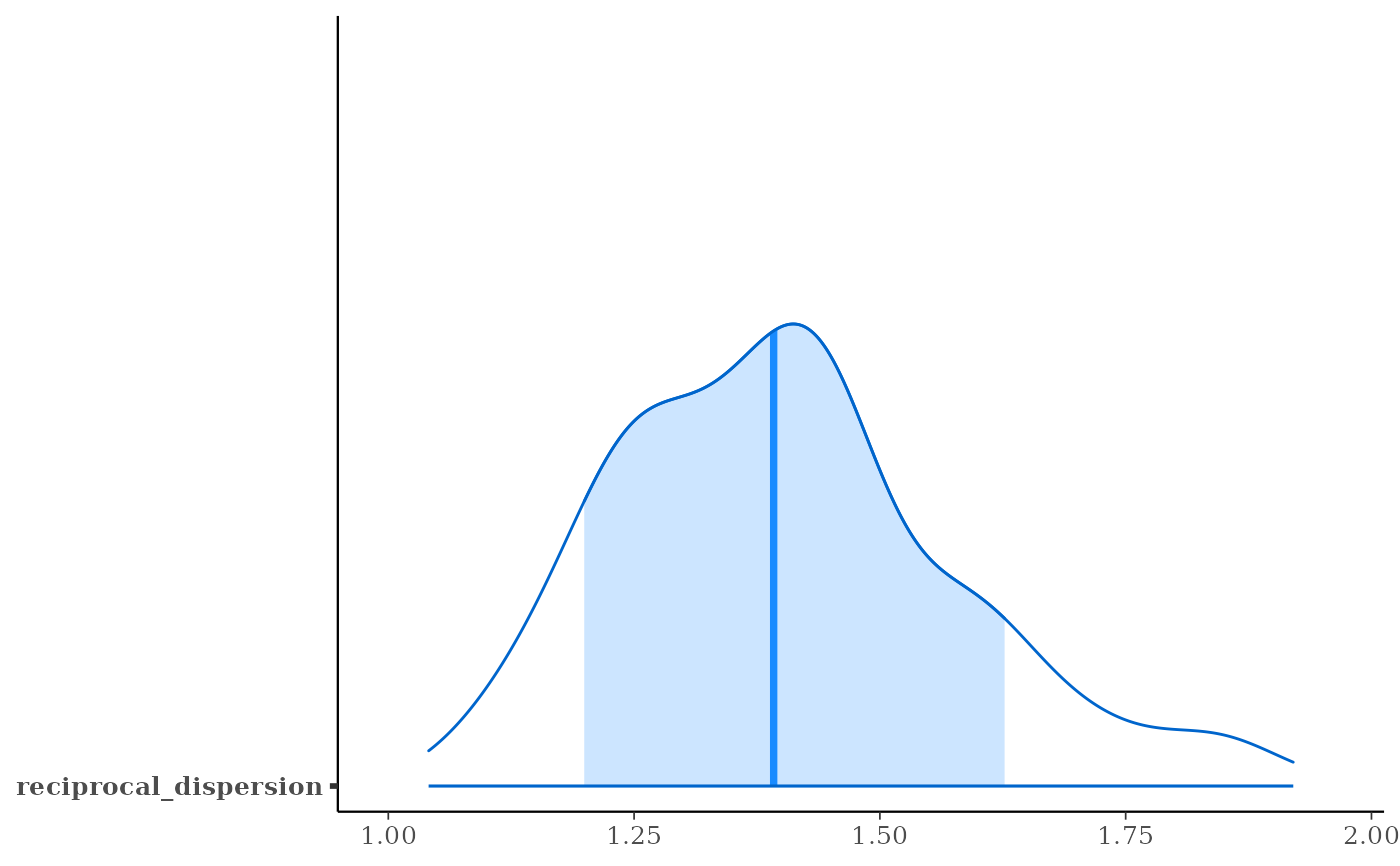
# 80% interval of estimated reciprocal_dispersion parameter
posterior_interval(fit6, pars = "reciprocal_dispersion", prob = 0.8)
plot(fit6, "areas", pars = "reciprocal_dispersion", prob = 0.8)
# }
}
#> Warning: The largest R-hat is 1.06, indicating chains have not mixed.
#> Running the chains for more iterations may help. See
#> https://mc-stan.org/misc/warnings.html#r-hat
#> Warning: Bulk Effective Samples Size (ESS) is too low, indicating posterior means and medians may be unreliable.
#> Running the chains for more iterations may help. See
#> https://mc-stan.org/misc/warnings.html#bulk-ess
#> Warning: Tail Effective Samples Size (ESS) is too low, indicating posterior variances and tail quantiles may be unreliable.
#> Running the chains for more iterations may help. See
#> https://mc-stan.org/misc/warnings.html#tail-ess
#> stan_glm
#>  family:       binomial [logit]
#>  formula:      switch ~ dist100 + arsenic
#>  observations: 3020
#>  predictors:   3
#> ------
#>             Median MAD_SD
#> (Intercept)  0.0    0.1  
#> dist100     -0.9    0.1  
#> arsenic      0.5    0.0  
#> 
#> ------
#> * For help interpreting the printed output see ?print.stanreg
#> * For info on the priors used see ?prior_summary.stanreg
#> 'x' not specified in '...'. Using x=1:length(y).
#> Warning: The largest R-hat is 1.07, indicating chains have not mixed.
#> Running the chains for more iterations may help. See
#> https://mc-stan.org/misc/warnings.html#r-hat
#> Warning: Bulk Effective Samples Size (ESS) is too low, indicating posterior means and medians may be unreliable.
#> Running the chains for more iterations may help. See
#> https://mc-stan.org/misc/warnings.html#bulk-ess
#> Warning: Tail Effective Samples Size (ESS) is too low, indicating posterior variances and tail quantiles may be unreliable.
#> Running the chains for more iterations may help. See
#> https://mc-stan.org/misc/warnings.html#tail-ess
#> stan_glm
#>  family:       poisson [log]
#>  formula:      counts ~ outcome + treatment
#>  observations: 9
#>  predictors:   5
#> ------
#>             Median MAD_SD
#> (Intercept)  3.0    0.2  
#> outcome2    -0.4    0.2  
#> outcome3    -0.3    0.2  
#> treatment2   0.0    0.2  
#> treatment3   0.0    0.2  
#> 
#> ------
#> * For help interpreting the printed output see ?print.stanreg
#> * For info on the priors used see ?prior_summary.stanreg
#> 
#> Drawing from prior...
#> Warning: Bulk Effective Samples Size (ESS) is too low, indicating posterior means and medians may be unreliable.
#> Running the chains for more iterations may help. See
#> https://mc-stan.org/misc/warnings.html#bulk-ess
#> stan_glm
#>  family:       Gamma [log]
#>  formula:      lot1 ~ log_u
#>  observations: 9
#>  predictors:   2
#> ------
#>             Median MAD_SD
#> (Intercept)  5.53   0.63 
#> log_u       -0.61   0.18 
#> 
#> Auxiliary parameter(s):
#>       Median MAD_SD
#> shape 3.93   1.82  
#> 
#> ------
#> * For help interpreting the printed output see ?print.stanreg
#> * For info on the priors used see ?prior_summary.stanreg
#> Warning: Bulk Effective Samples Size (ESS) is too low, indicating posterior means and medians may be unreliable.
#> Running the chains for more iterations may help. See
#> https://mc-stan.org/misc/warnings.html#bulk-ess
#> Warning: Bulk Effective Samples Size (ESS) is too low, indicating posterior means and medians may be unreliable.
#> Running the chains for more iterations may help. See
#> https://mc-stan.org/misc/warnings.html#bulk-ess
#> Warning: Tail Effective Samples Size (ESS) is too low, indicating posterior variances and tail quantiles may be unreliable.
#> Running the chains for more iterations may help. See
#> https://mc-stan.org/misc/warnings.html#tail-ess