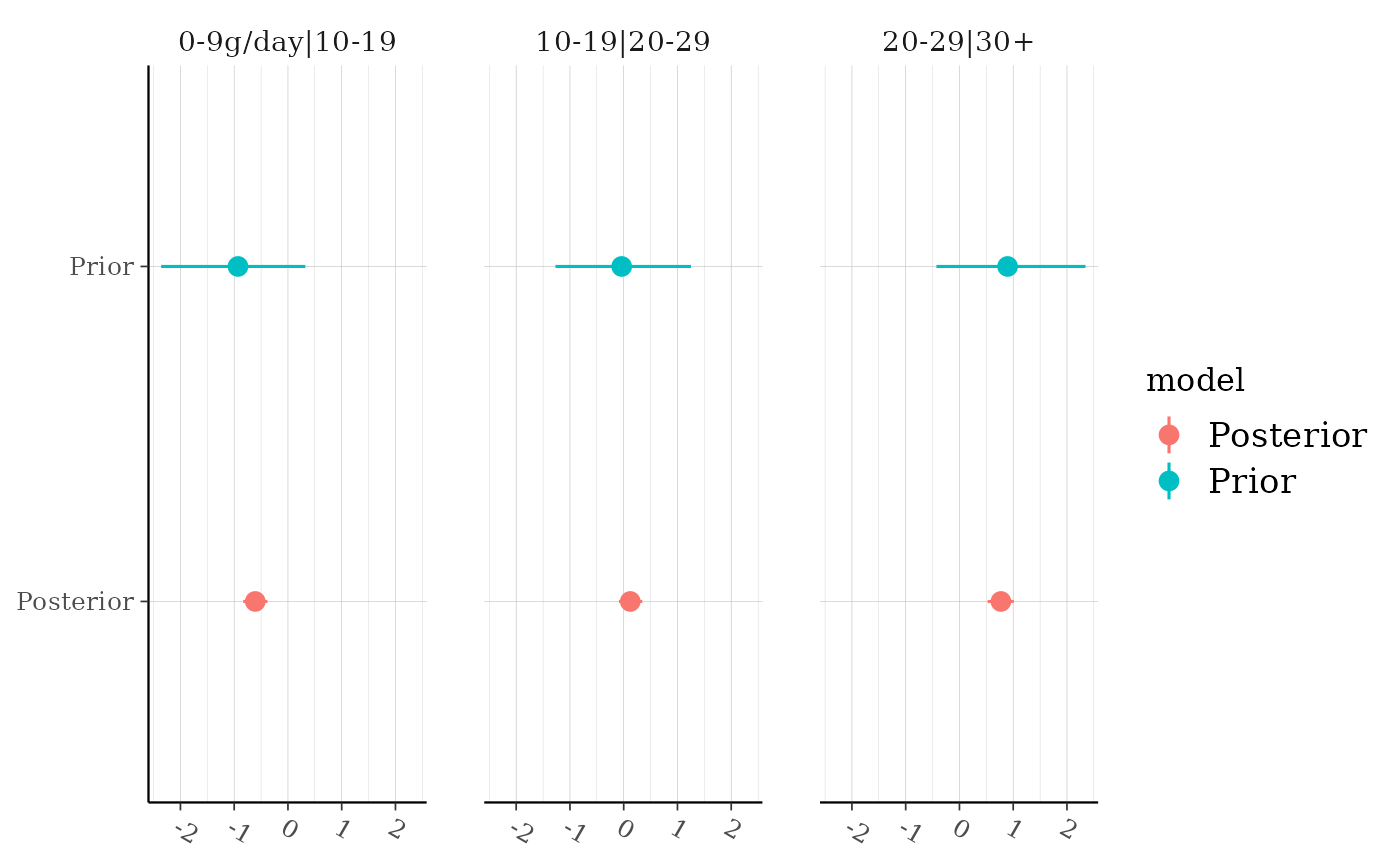
Plot medians and central intervals comparing parameter draws from the prior
and posterior distributions. If the plotted priors look different than the
priors you think you specified it is likely either because of internal
rescaling or the use of the QR argument (see the documentation for the
prior_summary method for details on
these special cases).
Arguments
- object
A fitted model object returned by one of the rstanarm modeling functions. See
stanreg-objects.- ...
The S3 generic uses
...to pass arguments to any defined methods. For the method for stanreg objects,...is for arguments (other thancolor) passed togeom_pointrangein the ggplot2 package to control the appearance of the plotted intervals.- pars
An optional character vector specifying a subset of parameters to display. Parameters can be specified by name or several shortcuts can be used. Using
pars="beta"will restrict the displayed parameters to only the regression coefficients (without the intercept)."alpha"can also be used as a shortcut for"(Intercept)". If the model has varying intercepts and/or slopes they can be selected usingpars = "varying".In addition, for
stanmvregobjects there are some additional shortcuts available. Usingpars = "long"will display the parameter estimates for the longitudinal submodels only (excluding group-specific pparameters, but including auxiliary parameters). Usingpars = "event"will display the parameter estimates for the event submodel only, including any association parameters. Usingpars = "assoc"will display only the association parameters. Usingpars = "fixef"will display all fixed effects, but not the random effects or the auxiliary parameters.parsandregex_parsare set toNULLthen all fixed effect regression coefficients are selected, as well as any auxiliary parameters and the log posterior.If
parsisNULLall parameters are selected for astanregobject, while for astanmvregobject all fixed effect regression coefficients are selected as well as any auxiliary parameters and the log posterior. See Examples.- regex_pars
An optional character vector of regular expressions to use for parameter selection.
regex_parscan be used in place ofparsor in addition topars. Currently, all functions that accept aregex_parsargument ignore it for models fit using optimization.- prob
A number \(p \in (0,1)\) indicating the desired posterior probability mass to include in the (central posterior) interval estimates displayed in the plot. The default is \(0.9\).
- color_by
How should the estimates be colored? Use
"parameter"to color by parameter name,"vs"to color the prior one color and the posterior another, and"none"to use no color. Except whencolor_by="none", a variable is mapped to the coloraesthetic and it is therefore also possible to change the default colors by adding one of the various discrete color scales available inggplot2(scale_color_manual,scale_colour_brewer, etc.). See Examples.- group_by_parameter
Should estimates be grouped together by parameter (
TRUE) or by posterior and prior (FALSE, the default)?- facet_args
A named list of arguments passed to
facet_wrap(other than thefacetsargument), e.g.,nroworncolto change the layout,scalesto allow axis scales to vary across facets, etc. See Examples.
References
Gabry, J. , Simpson, D. , Vehtari, A. , Betancourt, M. and Gelman, A. (2019), Visualization in Bayesian workflow. J. R. Stat. Soc. A, 182: 389-402. doi:10.1111/rssa.12378, arXiv preprint, code on GitHub)
Examples
if (.Platform$OS.type != "windows" || .Platform$r_arch != "i386") {
# \dontrun{
if (!exists("example_model")) example(example_model)
# display non-varying (i.e. not group-level) coefficients
posterior_vs_prior(example_model, pars = "beta")

# show group-level (varying) parameters and group by parameter
posterior_vs_prior(example_model, pars = "varying",
                   group_by_parameter = TRUE, color_by = "vs")

# group by parameter and allow axis scales to vary across facets
posterior_vs_prior(example_model, regex_pars = "period",
                   group_by_parameter = TRUE, color_by = "none",
                   facet_args = list(scales = "free"))

# assign to object and customize with functions from ggplot2
(gg <- posterior_vs_prior(example_model, pars = c("beta", "varying"), prob = 0.8))

gg +
 ggplot2::geom_hline(yintercept = 0, size = 0.3, linetype = 3) +
 ggplot2::coord_flip() +
 ggplot2::ggtitle("Comparing the prior and posterior")

# compare very wide and very narrow priors using roaches example
# (see help(roaches, "rstanarm") for info on the dataset)
roaches$roach100 <- roaches$roach1 / 100
wide_prior <- normal(0, 10)
narrow_prior <- normal(0, 0.1)
fit_pois_wide_prior <- stan_glm(y ~ treatment + roach100 + senior,
                                offset = log(exposure2),
                                family = "poisson", data = roaches,
                                prior = wide_prior)
posterior_vs_prior(fit_pois_wide_prior, pars = "beta", prob = 0.5,
                   group_by_parameter = TRUE, color_by = "vs",
                   facet_args = list(scales = "free"))

fit_pois_narrow_prior <- update(fit_pois_wide_prior, prior = narrow_prior)
posterior_vs_prior(fit_pois_narrow_prior, pars = "beta", prob = 0.5,
                   group_by_parameter = TRUE, color_by = "vs",
                   facet_args = list(scales = "free"))


# look at cutpoints for ordinal model
fit_polr <- stan_polr(tobgp ~ agegp, data = esoph, method = "probit",
                      prior = R2(0.2, "mean"), init_r = 0.1)
(gg_polr <- posterior_vs_prior(fit_polr, regex_pars = "\\|", color_by = "vs",
                               group_by_parameter = TRUE))
# flip the x and y axes
gg_polr + ggplot2::coord_flip()
# }
}
#>
#> Drawing from prior...
#>
#> Drawing from prior...
#>
#> Drawing from prior...
#>
#> Drawing from prior...
#> Warning: Using `size` aesthetic for lines was deprecated in ggplot2 3.4.0.
#> ℹ Please use `linewidth` instead.
#>
#> SAMPLING FOR MODEL 'count' NOW (CHAIN 1).
#> Chain 1:
#> Chain 1: Gradient evaluation took 3e-05 seconds
#> Chain 1: 1000 transitions using 10 leapfrog steps per transition would take 0.3 seconds.
#> Chain 1: Adjust your expectations accordingly!
#> Chain 1:
#> Chain 1:
#> Chain 1: Iteration:    1 / 2000 [  0%]  (Warmup)
#> Chain 1: Iteration:  200 / 2000 [ 10%]  (Warmup)
#> Chain 1: Iteration:  400 / 2000 [ 20%]  (Warmup)
#> Chain 1: Iteration:  600 / 2000 [ 30%]  (Warmup)
#> Chain 1: Iteration:  800 / 2000 [ 40%]  (Warmup)
#> Chain 1: Iteration: 1000 / 2000 [ 50%]  (Warmup)
#> Chain 1: Iteration: 1001 / 2000 [ 50%]  (Sampling)
#> Chain 1: Iteration: 1200 / 2000 [ 60%]  (Sampling)
#> Chain 1: Iteration: 1400 / 2000 [ 70%]  (Sampling)
#> Chain 1: Iteration: 1600 / 2000 [ 80%]  (Sampling)
#> Chain 1: Iteration: 1800 / 2000 [ 90%]  (Sampling)
#> Chain 1: Iteration: 2000 / 2000 [100%]  (Sampling)
#> Chain 1:
#> Chain 1:  Elapsed Time: 0.173 seconds (Warm-up)
#> Chain 1:                0.172 seconds (Sampling)
#> Chain 1:                0.345 seconds (Total)
#> Chain 1:
#>
#> SAMPLING FOR MODEL 'count' NOW (CHAIN 2).
#> Chain 2:
#> Chain 2: Gradient evaluation took 1.8e-05 seconds
#> Chain 2: 1000 transitions using 10 leapfrog steps per transition would take 0.18 seconds.
#> Chain 2: Adjust your expectations accordingly!
#> Chain 2:
#> Chain 2:
#> Chain 2: Iteration:    1 / 2000 [  0%]  (Warmup)
#> Chain 2: Iteration:  200 / 2000 [ 10%]  (Warmup)
#> Chain 2: Iteration:  400 / 2000 [ 20%]  (Warmup)
#> Chain 2: Iteration:  600 / 2000 [ 30%]  (Warmup)
#> Chain 2: Iteration:  800 / 2000 [ 40%]  (Warmup)
#> Chain 2: Iteration: 1000 / 2000 [ 50%]  (Warmup)
#> Chain 2: Iteration: 1001 / 2000 [ 50%]  (Sampling)
#> Chain 2: Iteration: 1200 / 2000 [ 60%]  (Sampling)
#> Chain 2: Iteration: 1400 / 2000 [ 70%]  (Sampling)
#> Chain 2: Iteration: 1600 / 2000 [ 80%]  (Sampling)
#> Chain 2: Iteration: 1800 / 2000 [ 90%]  (Sampling)
#> Chain 2: Iteration: 2000 / 2000 [100%]  (Sampling)
#> Chain 2:
#> Chain 2:  Elapsed Time: 0.198 seconds (Warm-up)
#> Chain 2:                0.232 seconds (Sampling)
#> Chain 2:                0.43 seconds (Total)
#> Chain 2:
#>
#> SAMPLING FOR MODEL 'count' NOW (CHAIN 3).
#> Chain 3:
#> Chain 3: Gradient evaluation took 1.7e-05 seconds
#> Chain 3: 1000 transitions using 10 leapfrog steps per transition would take 0.17 seconds.
#> Chain 3: Adjust your expectations accordingly!
#> Chain 3:
#> Chain 3:
#> Chain 3: Iteration:    1 / 2000 [  0%]  (Warmup)
#> Chain 3: Iteration:  200 / 2000 [ 10%]  (Warmup)
#> Chain 3: Iteration:  400 / 2000 [ 20%]  (Warmup)
#> Chain 3: Iteration:  600 / 2000 [ 30%]  (Warmup)
#> Chain 3: Iteration:  800 / 2000 [ 40%]  (Warmup)
#> Chain 3: Iteration: 1000 / 2000 [ 50%]  (Warmup)
#> Chain 3: Iteration: 1001 / 2000 [ 50%]  (Sampling)
#> Chain 3: Iteration: 1200 / 2000 [ 60%]  (Sampling)
#> Chain 3: Iteration: 1400 / 2000 [ 70%]  (Sampling)
#> Chain 3: Iteration: 1600 / 2000 [ 80%]  (Sampling)
#> Chain 3: Iteration: 1800 / 2000 [ 90%]  (Sampling)
#> Chain 3: Iteration: 2000 / 2000 [100%]  (Sampling)
#> Chain 3:
#> Chain 3:  Elapsed Time: 0.177 seconds (Warm-up)
#> Chain 3:                0.179 seconds (Sampling)
#> Chain 3:                0.356 seconds (Total)
#> Chain 3:
#>
#> SAMPLING FOR MODEL 'count' NOW (CHAIN 4).
#> Chain 4:
#> Chain 4: Gradient evaluation took 1.8e-05 seconds
#> Chain 4: 1000 transitions using 10 leapfrog steps per transition would take 0.18 seconds.
#> Chain 4: Adjust your expectations accordingly!
#> Chain 4:
#> Chain 4:
#> Chain 4: Iteration:    1 / 2000 [  0%]  (Warmup)
#> Chain 4: Iteration:  200 / 2000 [ 10%]  (Warmup)
#> Chain 4: Iteration:  400 / 2000 [ 20%]  (Warmup)
#> Chain 4: Iteration:  600 / 2000 [ 30%]  (Warmup)
#> Chain 4: Iteration:  800 / 2000 [ 40%]  (Warmup)
#> Chain 4: Iteration: 1000 / 2000 [ 50%]  (Warmup)
#> Chain 4: Iteration: 1001 / 2000 [ 50%]  (Sampling)
#> Chain 4: Iteration: 1200 / 2000 [ 60%]  (Sampling)
#> Chain 4: Iteration: 1400 / 2000 [ 70%]  (Sampling)
#> Chain 4: Iteration: 1600 / 2000 [ 80%]  (Sampling)
#> Chain 4: Iteration: 1800 / 2000 [ 90%]  (Sampling)
#> Chain 4: Iteration: 2000 / 2000 [100%]  (Sampling)
#> Chain 4:
#> Chain 4:  Elapsed Time: 0.181 seconds (Warm-up)
#> Chain 4:                0.162 seconds (Sampling)
#> Chain 4:                0.343 seconds (Total)
#> Chain 4:
#>
#> Drawing from prior...
#>
#> SAMPLING FOR MODEL 'count' NOW (CHAIN 1).
#> Chain 1:
#> Chain 1: Gradient evaluation took 2.8e-05 seconds
#> Chain 1: 1000 transitions using 10 leapfrog steps per transition would take 0.28 seconds.
#> Chain 1: Adjust your expectations accordingly!
#> Chain 1:
#> Chain 1:
#> Chain 1: Iteration:    1 / 2000 [  0%]  (Warmup)
#> Chain 1: Iteration:  200 / 2000 [ 10%]  (Warmup)
#> Chain 1: Iteration:  400 / 2000 [ 20%]  (Warmup)
#> Chain 1: Iteration:  600 / 2000 [ 30%]  (Warmup)
#> Chain 1: Iteration:  800 / 2000 [ 40%]  (Warmup)
#> Chain 1: Iteration: 1000 / 2000 [ 50%]  (Warmup)
#> Chain 1: Iteration: 1001 / 2000 [ 50%]  (Sampling)
#> Chain 1: Iteration: 1200 / 2000 [ 60%]  (Sampling)
#> Chain 1: Iteration: 1400 / 2000 [ 70%]  (Sampling)
#> Chain 1: Iteration: 1600 / 2000 [ 80%]  (Sampling)
#> Chain 1: Iteration: 1800 / 2000 [ 90%]  (Sampling)
#> Chain 1: Iteration: 2000 / 2000 [100%]  (Sampling)
#> Chain 1:
#> Chain 1:  Elapsed Time: 0.136 seconds (Warm-up)
#> Chain 1:                0.119 seconds (Sampling)
#> Chain 1:                0.255 seconds (Total)
#> Chain 1:
#>
#> SAMPLING FOR MODEL 'count' NOW (CHAIN 2).
#> Chain 2:
#> Chain 2: Gradient evaluation took 1.7e-05 seconds
#> Chain 2: 1000 transitions using 10 leapfrog steps per transition would take 0.17 seconds.
#> Chain 2: Adjust your expectations accordingly!
#> Chain 2:
#> Chain 2:
#> Chain 2: Iteration:    1 / 2000 [  0%]  (Warmup)
#> Chain 2: Iteration:  200 / 2000 [ 10%]  (Warmup)
#> Chain 2: Iteration:  400 / 2000 [ 20%]  (Warmup)
#> Chain 2: Iteration:  600 / 2000 [ 30%]  (Warmup)
#> Chain 2: Iteration:  800 / 2000 [ 40%]  (Warmup)
#> Chain 2: Iteration: 1000 / 2000 [ 50%]  (Warmup)
#> Chain 2: Iteration: 1001 / 2000 [ 50%]  (Sampling)
#> Chain 2: Iteration: 1200 / 2000 [ 60%]  (Sampling)
#> Chain 2: Iteration: 1400 / 2000 [ 70%]  (Sampling)
#> Chain 2: Iteration: 1600 / 2000 [ 80%]  (Sampling)
#> Chain 2: Iteration: 1800 / 2000 [ 90%]  (Sampling)
#> Chain 2: Iteration: 2000 / 2000 [100%]  (Sampling)
#> Chain 2:
#> Chain 2:  Elapsed Time: 0.121 seconds (Warm-up)
#> Chain 2:                0.12 seconds (Sampling)
#> Chain 2:                0.241 seconds (Total)
#> Chain 2:
#>
#> SAMPLING FOR MODEL 'count' NOW (CHAIN 3).
#> Chain 3:
#> Chain 3: Gradient evaluation took 1.8e-05 seconds
#> Chain 3: 1000 transitions using 10 leapfrog steps per transition would take 0.18 seconds.
#> Chain 3: Adjust your expectations accordingly!
#> Chain 3:
#> Chain 3:
#> Chain 3: Iteration:    1 / 2000 [  0%]  (Warmup)
#> Chain 3: Iteration:  200 / 2000 [ 10%]  (Warmup)
#> Chain 3: Iteration:  400 / 2000 [ 20%]  (Warmup)
#> Chain 3: Iteration:  600 / 2000 [ 30%]  (Warmup)
#> Chain 3: Iteration:  800 / 2000 [ 40%]  (Warmup)
#> Chain 3: Iteration: 1000 / 2000 [ 50%]  (Warmup)
#> Chain 3: Iteration: 1001 / 2000 [ 50%]  (Sampling)
#> Chain 3: Iteration: 1200 / 2000 [ 60%]  (Sampling)
#> Chain 3: Iteration: 1400 / 2000 [ 70%]  (Sampling)
#> Chain 3: Iteration: 1600 / 2000 [ 80%]  (Sampling)
#> Chain 3: Iteration: 1800 / 2000 [ 90%]  (Sampling)
#> Chain 3: Iteration: 2000 / 2000 [100%]  (Sampling)
#> Chain 3:
#> Chain 3:  Elapsed Time: 0.137 seconds (Warm-up)
#> Chain 3:                0.117 seconds (Sampling)
#> Chain 3:                0.254 seconds (Total)
#> Chain 3:
#>
#> SAMPLING FOR MODEL 'count' NOW (CHAIN 4).
#> Chain 4:
#> Chain 4: Gradient evaluation took 1.7e-05 seconds
#> Chain 4: 1000 transitions using 10 leapfrog steps per transition would take 0.17 seconds.
#> Chain 4: Adjust your expectations accordingly!
#> Chain 4:
#> Chain 4:
#> Chain 4: Iteration:    1 / 2000 [  0%]  (Warmup)
#> Chain 4: Iteration:  200 / 2000 [ 10%]  (Warmup)
#> Chain 4: Iteration:  400 / 2000 [ 20%]  (Warmup)
#> Chain 4: Iteration:  600 / 2000 [ 30%]  (Warmup)
#> Chain 4: Iteration:  800 / 2000 [ 40%]  (Warmup)
#> Chain 4: Iteration: 1000 / 2000 [ 50%]  (Warmup)
#> Chain 4: Iteration: 1001 / 2000 [ 50%]  (Sampling)
#> Chain 4: Iteration: 1200 / 2000 [ 60%]  (Sampling)
#> Chain 4: Iteration: 1400 / 2000 [ 70%]  (Sampling)
#> Chain 4: Iteration: 1600 / 2000 [ 80%]  (Sampling)
#> Chain 4: Iteration: 1800 / 2000 [ 90%]  (Sampling)
#> Chain 4: Iteration: 2000 / 2000 [100%]  (Sampling)
#> Chain 4:
#> Chain 4:  Elapsed Time: 0.132 seconds (Warm-up)
#> Chain 4:                0.106 seconds (Sampling)
#> Chain 4:                0.238 seconds (Total)
#> Chain 4:
#>
#> Drawing from prior...
#>
#> SAMPLING FOR MODEL 'polr' NOW (CHAIN 1).
#> Chain 1:
#> Chain 1: Gradient evaluation took 4.8e-05 seconds
#> Chain 1: 1000 transitions using 10 leapfrog steps per transition would take 0.48 seconds.
#> Chain 1: Adjust your expectations accordingly!
#> Chain 1:
#> Chain 1:
#> Chain 1: Iteration:    1 / 2000 [  0%]  (Warmup)
#> Chain 1: Iteration:  200 / 2000 [ 10%]  (Warmup)
#> Chain 1: Iteration:  400 / 2000 [ 20%]  (Warmup)
#> Chain 1: Iteration:  600 / 2000 [ 30%]  (Warmup)
#> Chain 1: Iteration:  800 / 2000 [ 40%]  (Warmup)
#> Chain 1: Iteration: 1000 / 2000 [ 50%]  (Warmup)
#> Chain 1: Iteration: 1001 / 2000 [ 50%]  (Sampling)
#> Chain 1: Iteration: 1200 / 2000 [ 60%]  (Sampling)
#> Chain 1: Iteration: 1400 / 2000 [ 70%]  (Sampling)
#> Chain 1: Iteration: 1600 / 2000 [ 80%]  (Sampling)
#> Chain 1: Iteration: 1800 / 2000 [ 90%]  (Sampling)
#> Chain 1: Iteration: 2000 / 2000 [100%]  (Sampling)
#> Chain 1:
#> Chain 1:  Elapsed Time: 0.579 seconds (Warm-up)
#> Chain 1:                0.519 seconds (Sampling)
#> Chain 1:                1.098 seconds (Total)
#> Chain 1:
#>
#> SAMPLING FOR MODEL 'polr' NOW (CHAIN 2).
#> Chain 2:
#> Chain 2: Gradient evaluation took 3.5e-05 seconds
#> Chain 2: 1000 transitions using 10 leapfrog steps per transition would take 0.35 seconds.
#> Chain 2: Adjust your expectations accordingly!
#> Chain 2:
#> Chain 2:
#> Chain 2: Iteration:    1 / 2000 [  0%]  (Warmup)
#> Chain 2: Iteration:  200 / 2000 [ 10%]  (Warmup)
#> Chain 2: Iteration:  400 / 2000 [ 20%]  (Warmup)
#> Chain 2: Iteration:  600 / 2000 [ 30%]  (Warmup)
#> Chain 2: Iteration:  800 / 2000 [ 40%]  (Warmup)
#> Chain 2: Iteration: 1000 / 2000 [ 50%]  (Warmup)
#> Chain 2: Iteration: 1001 / 2000 [ 50%]  (Sampling)
#> Chain 2: Iteration: 1200 / 2000 [ 60%]  (Sampling)
#> Chain 2: Iteration: 1400 / 2000 [ 70%]  (Sampling)
#> Chain 2: Iteration: 1600 / 2000 [ 80%]  (Sampling)
#> Chain 2: Iteration: 1800 / 2000 [ 90%]  (Sampling)
#> Chain 2: Iteration: 2000 / 2000 [100%]  (Sampling)
#> Chain 2:
#> Chain 2:  Elapsed Time: 0.54 seconds (Warm-up)
#> Chain 2:                0.452 seconds (Sampling)
#> Chain 2:                0.992 seconds (Total)
#> Chain 2:
#>
#> SAMPLING FOR MODEL 'polr' NOW (CHAIN 3).
#> Chain 3:
#> Chain 3: Gradient evaluation took 3.6e-05 seconds
#> Chain 3: 1000 transitions using 10 leapfrog steps per transition would take 0.36 seconds.
#> Chain 3: Adjust your expectations accordingly!
#> Chain 3:
#> Chain 3:
#> Chain 3: Iteration:    1 / 2000 [  0%]  (Warmup)
#> Chain 3: Iteration:  200 / 2000 [ 10%]  (Warmup)
#> Chain 3: Iteration:  400 / 2000 [ 20%]  (Warmup)
#> Chain 3: Iteration:  600 / 2000 [ 30%]  (Warmup)
#> Chain 3: Iteration:  800 / 2000 [ 40%]  (Warmup)
#> Chain 3: Iteration: 1000 / 2000 [ 50%]  (Warmup)
#> Chain 3: Iteration: 1001 / 2000 [ 50%]  (Sampling)
#> Chain 3: Iteration: 1200 / 2000 [ 60%]  (Sampling)
#> Chain 3: Iteration: 1400 / 2000 [ 70%]  (Sampling)
#> Chain 3: Iteration: 1600 / 2000 [ 80%]  (Sampling)
#> Chain 3: Iteration: 1800 / 2000 [ 90%]  (Sampling)
#> Chain 3: Iteration: 2000 / 2000 [100%]  (Sampling)
#> Chain 3:
#> Chain 3:  Elapsed Time: 0.544 seconds (Warm-up)
#> Chain 3:                0.489 seconds (Sampling)
#> Chain 3:                1.033 seconds (Total)
#> Chain 3:
#>
#> SAMPLING FOR MODEL 'polr' NOW (CHAIN 4).
#> Chain 4:
#> Chain 4: Gradient evaluation took 3.5e-05 seconds
#> Chain 4: 1000 transitions using 10 leapfrog steps per transition would take 0.35 seconds.
#> Chain 4: Adjust your expectations accordingly!
#> Chain 4:
#> Chain 4:
#> Chain 4: Iteration:    1 / 2000 [  0%]  (Warmup)
#> Chain 4: Iteration:  200 / 2000 [ 10%]  (Warmup)
#> Chain 4: Iteration:  400 / 2000 [ 20%]  (Warmup)
#> Chain 4: Iteration:  600 / 2000 [ 30%]  (Warmup)
#> Chain 4: Iteration:  800 / 2000 [ 40%]  (Warmup)
#> Chain 4: Iteration: 1000 / 2000 [ 50%]  (Warmup)
#> Chain 4: Iteration: 1001 / 2000 [ 50%]  (Sampling)
#> Chain 4: Iteration: 1200 / 2000 [ 60%]  (Sampling)
#> Chain 4: Iteration: 1400 / 2000 [ 70%]  (Sampling)
#> Chain 4: Iteration: 1600 / 2000 [ 80%]  (Sampling)
#> Chain 4: Iteration: 1800 / 2000 [ 90%]  (Sampling)
#> Chain 4: Iteration: 2000 / 2000 [100%]  (Sampling)
#> Chain 4:
#> Chain 4:  Elapsed Time: 0.555 seconds (Warm-up)
#> Chain 4:                0.462 seconds (Sampling)
#> Chain 4:                1.017 seconds (Total)
#> Chain 4:
#>
#> Drawing from prior...