27.3 Posterior ``p-values’’
If a model captures the data well, summary statistics such as sample mean and standard deviation, should have similar values in the original and replicated data sets. This can be tested by means of a p-value-like statistic, which here is just the probability the test statistic \(s(\cdot)\) in a replicated data set exceeds that in the original data, \[ \textrm{Pr}\left[ s(y^{\textrm{rep}}) \geq s(y) \mid y \right] = \int \textrm{I}\left( s(y^{\textrm{rep}}) \geq s(y) \mid y \right) \cdot p\left( y^{\textrm{rep}} \mid y \right) \, \textrm{d}{y^{\textrm{rep}}}. \] It is important to note that``p-values’’ is in quotes because these statistics are not classically calibrated, and thus will not in general have a uniform distribution even when the model is well specified (Bayarri and Berger 2000).
Nevertheless, values of this statistic very close to zero or one are cause for concern that the model is not fitting the data well. Unlike a visual test, this p-value-like test is easily automated for bulk model fitting.
To calculate event probabilities in Stan, it suffices to define indicator variables that take on value 1 if the event occurs and 0 if it does not. The posterior mean is then the event probability. For efficiency, indicator variables are defined in the generated quantities block.
generated quantities {
  int<lower = 0, upper = 1> mean_gt;
  int<lower = 0, upper = 1> sd_gt;
  {
    real y_rep[N] = normal_rng(alpha + beta * x, sigma);
    mean_gt = mean(y_rep) > mean(y);
    sd_gt = sd(y_rep) > sd(y);
  }
}
The indicator variable mean_gt will have value 1 if the mean of the
simulated data y_rep is greater than or equal to the mean of he
original data y. Because the values of y_rep are not needed for
the posterior predictive checks, the program saves output space by
using a local variable for y_rep. The statistics mean(u) and
sd(y) could also be computed in the transformed data block and
saved.
For the example in the previous section, where over-dispersed data generated by a negative binomial distribution was fit with a simple Poisson model, the following plot illustrates the posterior p-value calculation for the mean statistic.
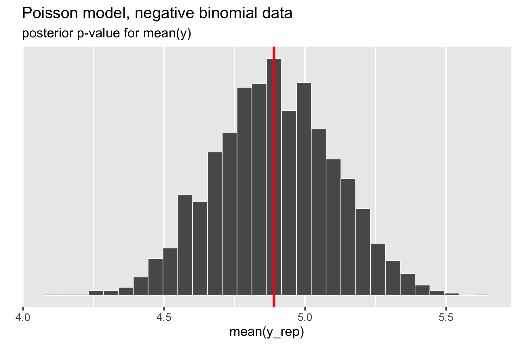
Figure 27.3: Histogram of means of replicated data sets; vertical red line at mean of original data.
The p-value for the mean is just the percentage of replicated data
sets whose statistic is greater than or equal that of the original
data. Using a Poisson model for negative binomial data still fits the
mean well, with a posterior \(p\)-value of 0.49. In Stan terms, it is
extracted as the posterior mean of the indicator variable mean_gt.
The standard deviation statistic tells a different story.
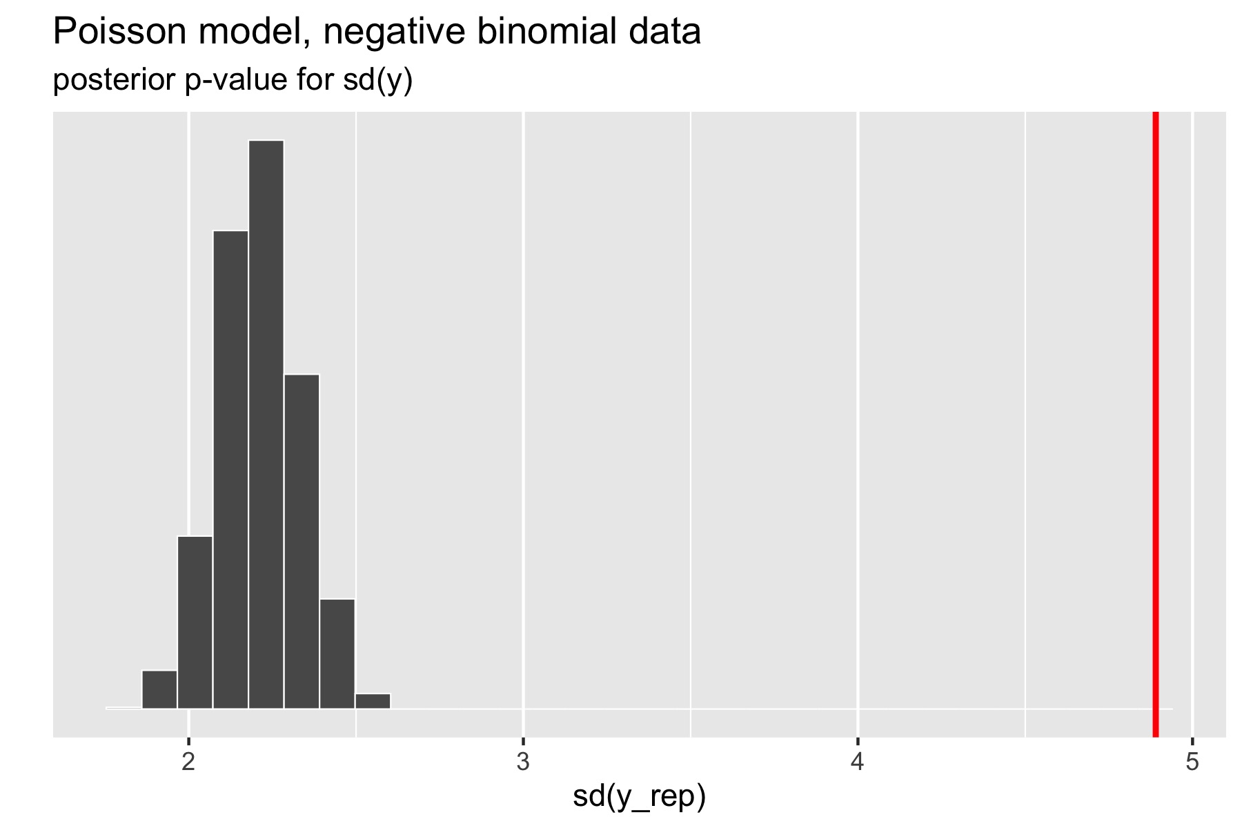
Figure 27.4: Scatterplot of standard deviations of replicated data sets; the vertical red line is at standard deviation of original data.
Here, the original data has much higher standard deviation than any of the replicated data sets. The resulting \(p\)-value estimated by Stan after a large number of iterations is exactly zero (the absolute error bounds are fine, but a lot of iterations are required to get good relative error bounds on small \(p\)-values by sampling). In other words, there were no posterior draws in which the replicated data set had a standard deviation greater than or equal to that of the original data set. Clearly, the model is not capturing the dispersion of the original data. The point of this exercise isn’t just to figure out that there’s a problem with a model, but to isolate where it is. Seeing that the data is over-dispersed compared to the Poisson model would be reason to fit a more general model like the negative binomial or a latent varying effects (aka random effects) model that can account for the over-dispersion.
27.3.1 Which statistics to test?
Any statistic may be used for the data, but these can be guided by the quantities of interest in the model itself. Popular choices in addition to mean and standard deviation are quantiles, such as the median, 5% or 95% quantiles, or even the maximum or minimum value to test extremes.
Despite the range of choices, test statistics should ideally be ancillary, in the sense that they should be testing something other than the fit of a parameter. For example, a simple normal model of a data set will typically fit the mean and variance of the data quite well as long as the prior doesn’t dominate the posterior. In contrast, a Poisson model of the same data cannot capture both the mean and the variance of a data set if they are different, so they bear checking in the Poisson case. As we saw with the Poisson case, the posterior mean for the single rate parameter was located near the data mean, not the data variance. Other distributions such as the lognormal and gamma distribution, have means and variances that are functions of two or more parameters.