23.7 Reparameterization
Stan’s sampler can be slow in sampling from distributions with difficult posterior geometries. One way to speed up such models is through reparameterization. In some cases, reparameterization can dramatically increase effective sample size for the same number of iterations or even make programs that would not converge well behaved.
Example: Neal’s funnel
In this section, we discuss a general transform from a centered to a non-centered parameterization (Papaspiliopoulos, Roberts, and Sköld 2007).39
This reparameterization is helpful when there is not much data, because it separates the hierarchical parameters and lower-level parameters in the prior.
Neal (2003) defines a distribution that exemplifies the difficulties of sampling from some hierarchical models. Neal’s example is fairly extreme, but can be trivially reparameterized in such a way as to make sampling straightforward. Neal’s example has support for \(y \in \mathbb{R}\) and \(x \in \mathbb{R}^9\) with density
\[ p(y,x) = \textsf{normal}(y \mid 0,3) \times \prod_{n=1}^9 \textsf{normal}(x_n \mid 0,\exp(y/2)). \]
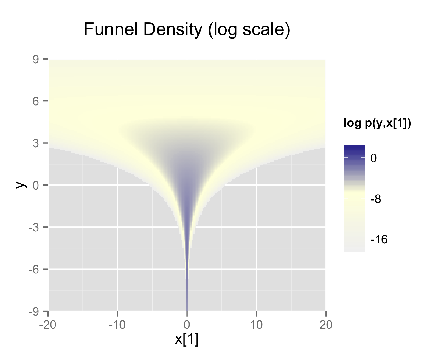
The probability contours are shaped like ten-dimensional funnels. The funnel’s neck is particularly sharp because of the exponential function applied to \(y\). A plot of the log marginal density of \(y\) and the first dimension \(x_1\) is shown in the following plot.
The marginal density of Neal’s funnel for the upper-level variable \(y\) and one lower-level variable \(x_1\) (see the text for the formula). The blue region has log density greater than -8, the yellow region density greater than -16, and the gray background a density less than -16.
Neal’s funnel density
The funnel can be implemented directly in Stan as follows.
parameters {
real y;
vector[9] x;
}
model {
y ~ normal(0, 3);
x ~ normal(0, exp(y/2));
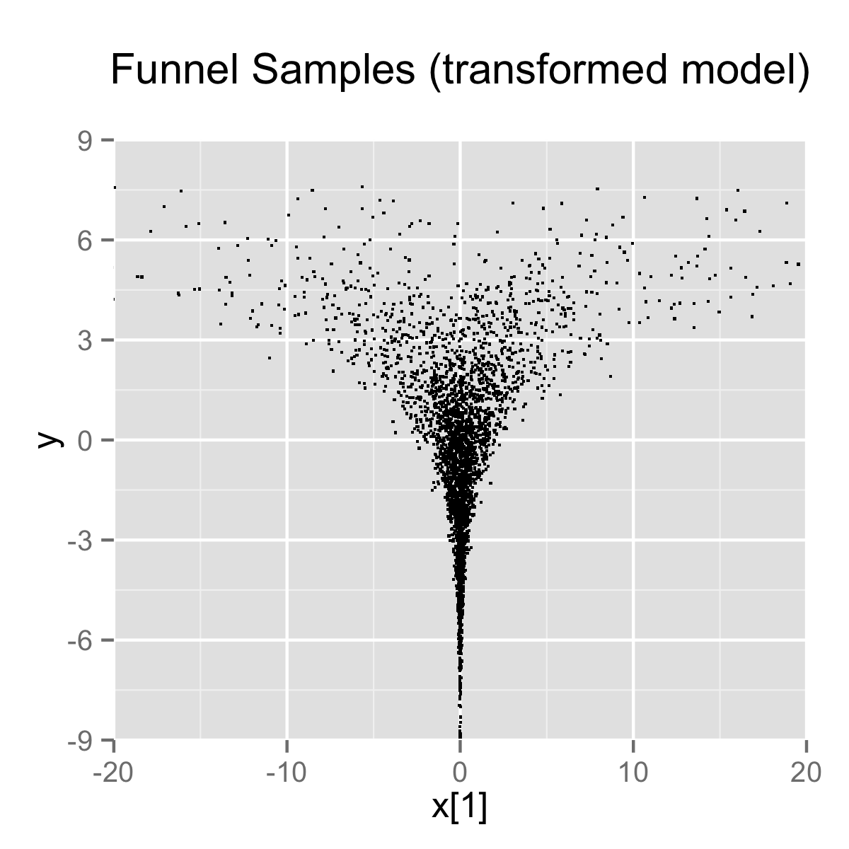
}When the model is expressed this way, Stan has trouble sampling from the neck of the funnel, where \(y\) is small and thus \(x\) is constrained to be near 0. This is due to the fact that the density’s scale changes with \(y\), so that a step size that works well in the body will be too large for the neck, and a step size that works in the neck will be inefficient in the body. This can be seen in the following plot.
4000 draws are taken from a run of Stan’s sampler with default settings. Both plots are restricted to the shown window of \(x_1\) and \(y\) values; some draws fell outside of the displayed area as would be expected given the density. The samples are consistent with the marginal density \(p(y) = \textsf{normal}(y \mid 0,3)\), which has mean 0 and standard deviation 3.
In this particular instance, because the analytic form of the density from which samples are drawn is known, the model can be converted to the following more efficient form.
parameters {
  real y_raw;
  vector[9] x_raw;
}
transformed parameters {
  real y;
  vector[9] x;

  y = 3.0 * y_raw;
  x = exp(y/2) * x_raw;
}
model {
  y_raw ~ std_normal(); // implies y ~ normal(0, 3)
  x_raw ~ std_normal(); // implies x ~ normal(0, exp(y/2))
}
In this second model, the parameters x_raw and y_raw are
sampled as independent standard normals, which is easy for Stan. These
are then transformed into samples from the funnel. In this case, the
same transform may be used to define Monte Carlo samples directly
based on independent standard normal samples; Markov chain Monte Carlo
methods are not necessary. If such a reparameterization were used in
Stan code, it is useful to provide a comment indicating what the
distribution for the parameter implies for the distribution of the
transformed parameter.
Reparameterizing the Cauchy
Sampling from heavy tailed distributions such as the Cauchy is difficult for Hamiltonian Monte Carlo, which operates within a Euclidean geometry.40
The practical problem is that tail of the Cauchy requires a relatively large step size compared to the trunk. With a small step size, the No-U-Turn sampler requires many steps when starting in the tail of the distribution; with a large step size, there will be too much rejection in the central portion of the distribution. This problem may be mitigated by defining the Cauchy-distributed variable as the transform of a uniformly distributed variable using the Cauchy inverse cumulative distribution function.
Suppose a random variable of interest \(X\) has a Cauchy distribution with location \(\mu\) and scale \(\tau\), so that \(X \sim \textsf{Cauchy}(\mu,\tau)\). The variable \(X\) has a cumulative distribution function \(F_X:\mathbb{R} \rightarrow (0,1)\) defined by \[ F_X(x) = \frac{1}{\pi} \arctan \left( \frac{x - \mu}{\tau} \right) + \frac{1}{2}. \] The inverse of the cumulative distribution function, \(F_X^{-1}:(0,1) \rightarrow \mathbb{R}\), is thus
\[ F^{-1}_X(y) = \mu + \tau \tan \left( \pi \left( y - \frac{1}{2} \right) \right). \] Thus if the random variable \(Y\) has a unit uniform distribution, \(Y \sim \textsf{uniform}(0,1)\), then \(F^{-1}_X(Y)\) has a Cauchy distribution with location \(\mu\) and scale \(\tau\), i.e., \(F^{-1}_X(Y) \sim \textsf{Cauchy}(\mu,\tau)\).
Consider a Stan program involving a Cauchy-distributed parameter
beta.
parameters {
  real beta;
  ...
}
model {
  beta ~ cauchy(mu, tau);
  ...
}
This declaration of beta as a parameter may be replaced with a
transformed parameter beta defined in terms of a
uniform-distributed parameter beta_unif.
parameters {
  real<lower = -pi()/2, upper = pi()/2> beta_unif;
  ...
}
transformed parameters {
  real beta;
  beta = mu + tau * tan(beta_unif);  // beta ~ cauchy(mu, tau)
}
model {
  beta_unif ~ uniform(-pi()/2, pi()/2);  // not necessary
  ...
}
It is more convenient in Stan to transform a uniform variable on
\((-\pi/2, \pi/2)\) than one on \((0,1)\). The Cauchy location and scale
parameters, mu and tau, may be defined as data or may
themselves be parameters. The variable beta could also be
defined as a local variable if it does not need to be included in the
sampler’s output.
The uniform distribution on beta_unif is defined explicitly in
the model block, but it could be safely removed from the program
without changing sampling behavior. This is because \(\log \textsf{uniform}(\beta_{\textsf{unif}} \mid -\pi/2,\pi/2) = -\log \pi\) is a constant and Stan only
needs the total log probability up to an additive constant. Stan will spend
some time checking that that beta_unif is between
-pi()/2 and pi()/2, but this condition is guaranteed by
the constraints in the declaration of beta_unif.
Reparameterizing a Student-t distribution
One thing that sometimes works when you’re having trouble with the heavy-tailedness of Student-t distributions is to use the gamma-mixture representation, which says that you can generate a Student-t distributed variable \(\beta\), \[ \beta \sim \textsf{Student-t}(\nu, 0, 1), \] by first generating a gamma-distributed precision (inverse variance) \(\tau\) according to \[ \tau \sim \textsf{Gamma}(\nu/2, \nu/2), \] and then generating \(\beta\) from the normal distribution, \[ \beta \sim \textsf{normal}\left(0,\tau^{-\frac{1}{2}}\right). \]
Because \(\tau\) is precision, \(\tau^{-\frac{1}{2}}\) is the scale (standard deviation), which is the parameterization used by Stan.
The marginal distribution of \(\beta\) when you integrate out \(\tau\) is \(\textsf{Student-t}(\nu, 0, 1)\), i.e., \[ \textsf{Student-t}(\beta \mid \nu, 0, 1) = \int_0^{\infty} \, \textsf{normal}\left(\beta \middle| 0, \tau^{-0.5}\right) \times \textsf{Gamma}\left(\tau \middle| \nu/2, \nu/2\right) \ \textsf{d} \tau. \]
To go one step further, instead of defining a \(\beta\) drawn from a normal with precision \(\tau\), define \(\alpha\) to be drawn from a unit normal, \[ \alpha \sim \textsf{normal}(0,1) \] and rescale by defining \[ \beta = \alpha \, \tau^{-\frac{1}{2}}. \]
Now suppose \(\mu = \beta x\) is the product of \(\beta\) with a regression predictor \(x\). Then the reparameterization \(\mu = \alpha \tau^{-\frac{1}{2}} x\) has the same distribution, but in the original, direct parameterization, \(\beta\) has (potentially) heavy tails, whereas in the second, neither \(\tau\) nor \(\alpha\) have heavy tails.
To translate into Stan notation, this reparameterization replaces
parameters {
  real<lower=0> nu;
  real beta;
  ...
model {
  beta ~ student_t(nu, 0, 1);
  ...
with
parameters {
  real<lower=0> nu;
  real<lower=0> tau;
  real alpha;
  ...
transformed parameters {
  real beta;
  beta = alpha / sqrt(tau);
  ...
model {
  real half_nu;
  half_nu = 0.5 * nu;
  tau ~ gamma(half_nu, half_nu);
  alpha ~ std_normal();
  ...
Although set to 0 here, in most cases, the lower bound for the
degrees of freedom parameter nu can be set to 1 or
higher; when nu is 1, the result is a Cauchy distribution with
fat tails and as nu approaches infinity, the Student-t
distribution approaches a normal distribution. Thus the parameter
nu characterizes the heaviness of the tails of the model.
Hierarchical models and the non-centered parameterization
Unfortunately, the usual situation in applied Bayesian modeling involves complex geometries and interactions that are not known analytically. Nevertheless, reparameterization can still be effective for separating parameters.
Centered parameterization
For example, a vectorized hierarchical model might draw a vector of coefficients \(\beta\) with definitions as follows. The so-called centered parameterization is as follows.
parameters {
  real mu_beta;
  real<lower = 0> sigma_beta;
  vector[K] beta;
  ...
model {
  beta ~ normal(mu_beta, sigma_beta);
  ...
Although not shown, a full model will have priors on both
mu_beta and sigma_beta along with data modeled based on
these coefficients. For instance, a standard binary logistic
regression with data matrix x and binary outcome vector
y would include a likelihood statement such as form
y ~ bernoulli_logit(x * beta), leading to an analytically
intractable posterior.
A hierarchical model such as the above will suffer from the same kind
of inefficiencies as Neal’s funnel, because the values of beta,
mu_beta and sigma_beta are highly correlated in the
posterior. The extremity of the correlation depends on the amount of
data, with Neal’s funnel being the extreme with no data. In these
cases, the non-centered parameterization, discussed in the next
section, is preferable; when there is a lot of data, the centered
parameterization is more efficient. See
Betancourt and Girolami (2013) for more information on the effects of
centering in hierarchical models fit with Hamiltonian Monte Carlo.
Non-centered parameterization
Sometimes the group-level effects do not constrain the hierarchical distribution tightly. Examples arise when there are not many groups, or when the inter-group variation is high. In such cases, hierarchical models can be made much more efficient by shifting the data’s correlation with the parameters to the hyperparameters. Similar to the funnel example, this will be much more efficient in terms of effective sample size when there is not much data (see Betancourt and Girolami (2013)), and in more extreme cases will be necessary to achieve convergence.
parameters {
  vector[K] beta_raw;
  ...
transformed parameters {
  vector[K] beta;
  // implies: beta ~ normal(mu_beta, sigma_beta)
  beta = mu_beta + sigma_beta * beta_raw;
model {
  beta_raw ~ std_normal();
  ...
Any priors defined for mu_beta and sigma_beta remain as
defined in the original model.
Reparameterization of hierarchical models is not limited to the normal distribution, although the normal distribution is the best candidate for doing so. In general, any distribution of parameters in the location-scale family is a good candidate for reparameterization. Let \(\beta = l + s\alpha\) where \(l\) is a location parameter and \(s\) is a scale parameter. The parameter \(l\) need not be the mean, \(s\) need not be the standard deviation, and neither the mean nor the standard deviation need to exist. If \(\alpha\) and \(\beta\) are from the same distributional family but \(\alpha\) has location zero and unit scale, while \(\beta\) has location \(l\) and scale \(s\), then that distribution is a location-scale distribution. Thus, if \(\alpha\) were a parameter and \(\beta\) were a transformed parameter, then a prior distribution from the location-scale family on \(\alpha\) with location zero and unit scale implies a prior distribution on \(\beta\) with location \(l\) and scale \(s\). Doing so would reduce the dependence between \(\alpha\), \(l\), and \(s\).
There are several univariate distributions in the location-scale family, such as the Student t distribution, including its special cases of the Cauchy distribution (with one degree of freedom) and the normal distribution (with infinite degrees of freedom). As shown above, if \(\alpha\) is distributed standard normal, then \(\beta\) is distributed normal with mean \(\mu = l\) and standard deviation \(\sigma = s\). The logistic, the double exponential, the generalized extreme value distributions, and the stable distribution are also in the location-scale family.
Also, if \(z\) is distributed standard normal, then \(z^2\) is distributed chi-squared with one degree of freedom. By summing the squares of \(K\) independent standard normal variates, one can obtain a single variate that is distributed chi-squared with \(K\) degrees of freedom. However, for large \(K\), the computational gains of this reparameterization may be overwhelmed by the computational cost of specifying \(K\) primitive parameters just to obtain one transformed parameter to use in a model.
Multivariate reparameterizations
The benefits of reparameterization are not limited to univariate distributions. A parameter with a multivariate normal prior distribution is also an excellent candidate for reparameterization. Suppose you intend the prior for \(\beta\) to be multivariate normal with mean vector \(\mu\) and covariance matrix \(\Sigma\). Such a belief is reflected by the following code.
data {
  int<lower=2> K;
  vector[K] mu;
  cov_matrix[K] Sigma;
  ...
parameters {
  vector[K] beta;
  ...
model {
  beta ~ multi_normal(mu, Sigma);
  ...
In this case mu and Sigma are fixed data, but they could
be unknown parameters, in which case their priors would be unaffected
by a reparameterization of beta.
If \(\alpha\) has the same dimensions as \(\beta\) but the elements of \(\alpha\) are independently and identically distributed standard normal such that \(\beta = \mu + L\alpha\), where \(LL^\top = \Sigma\), then \(\beta\) is distributed multivariate normal with mean vector \(\mu\) and covariance matrix \(\Sigma\). One choice for \(L\) is the Cholesky factor of \(\Sigma\). Thus, the model above could be reparameterized as follows.
data {
  int<lower=2> K;
  vector[K] mu;
  cov_matrix[K] Sigma;
  ...
transformed data {
  matrix[K, K] L;
  L = cholesky_decompose(Sigma);
}
parameters {
  vector[K] alpha;
  ...
transformed parameters {
  vector[K] beta;
  beta = mu + L * alpha;
}
model {
  alpha ~ std_normal();
  // implies: beta ~ multi_normal(mu, Sigma)
  ...
This reparameterization is more efficient for two reasons. First, it
reduces dependence among the elements of alpha and second, it
avoids the need to invert Sigma every time multi_normal
is evaluated.
The Cholesky factor is also useful when a covariance matrix is
decomposed into a correlation matrix that is multiplied from both
sides by a diagonal matrix of standard deviations, where either the
standard deviations or the correlations are unknown parameters. The
Cholesky factor of the covariance matrix is equal to the product of
a diagonal matrix of standard deviations and the Cholesky factor of
the correlation matrix. Furthermore, the product of a diagonal matrix
of standard deviations and a vector is equal to the elementwise
product between the standard deviations and that vector. Thus, if for
example the correlation matrix Tau were fixed data but the
vector of standard deviations sigma were unknown parameters,
then a reparameterization of beta in terms of alpha
could be implemented as follows.
data {
  int<lower=2> K;
  vector[K] mu;
  corr_matrix[K] Tau;
  ...
transformed data {
  matrix[K, K] L;
  L = cholesky_decompose(Tau);
}
parameters {
  vector[K] alpha;
  vector<lower=0>[K] sigma;
  ...
transformed parameters {
  vector[K] beta;
  // This equals mu + diag_matrix(sigma) * L * alpha;
  beta = mu + sigma .* (L * alpha);
}
model {
  sigma ~ cauchy(0, 5);
  alpha ~ std_normal();
  // implies: beta ~ multi_normal(mu,
  //  diag_matrix(sigma) * L * L' * diag_matrix(sigma)))
  ...
This reparameterization of a multivariate normal distribution in terms of standard normal variates can be extended to other multivariate distributions that can be conceptualized as contaminations of the multivariate normal, such as the multivariate Student t and the skew multivariate normal distribution.
A Wishart distribution can also be reparameterized in terms of standard normal variates and chi-squared variates. Let \(L\) be the Cholesky factor of a \(K \times K\) positive definite scale matrix \(S\) and let \(\nu\) be the degrees of freedom. If \[ A = \begin{pmatrix} \sqrt{c_{1}} & 0 & \cdots & 0 \\ z_{21} & \sqrt{c_{2}} & \ddots & \vdots \\ \vdots & \ddots & \ddots & 0 \\ z_{K1} & \cdots & z_{K\left(K-1\right)} & \sqrt{c_{K}} \end{pmatrix}, \] where each \(c_i\) is distributed chi-squared with \(\nu - i + 1\) degrees of freedom and each \(z_{ij}\) is distributed standard normal, then \(W = LAA^{\top}L^{\top}\) is distributed Wishart with scale matrix \(S = LL^{\top}\) and degrees of freedom \(\nu\). Such a reparameterization can be implemented by the following Stan code:
data {
  int<lower=1> N;
  int<lower=1> K;
  int<lower=K+2> nu
  matrix[K, K] L; // Cholesky factor of scale matrix
  vector[K] mu;
  matrix[N, K] y;
  ...
parameters {
  vector<lower=0>[K] c;
  vector[0.5 * K * (K - 1)] z;
  ...
model {
  matrix[K, K] A;
  int count = 1;
  for (j in 1:(K-1)) {
    for (i in (j+1):K) {
      A[i, j] = z[count];
      count += 1;
    }
    for (i in 1:(j - 1)) {
      A[i, j] = 0.0;
    }
    A[j, j] = sqrt(c[j]);
  }
  for (i in 1:(K-1))
    A[i, K] = 0;
  A[K, K] = sqrt(c[K]);

  for (i in 1:K)
    c[i] ~ chi_square(nu - i + 1);

  z ~ std_normal();
  // implies: L * A * A' * L' ~ wishart(nu, L * L')
  y ~ multi_normal_cholesky(mu, L * A);
  ...
This reparameterization is more efficient for three reasons. First, it
reduces dependence among the elements of z and second, it
avoids the need to invert the covariance matrix, \(W\) every time
wishart is evaluated. Third, if \(W\) is to be used with a
multivariate normal distribution, you can pass \(L A\) to the more
efficient multi_normal_cholesky function, rather than passing
\(W\) to multi_normal.
If \(W\) is distributed Wishart with scale matrix \(S\) and degrees of freedom \(\nu\), then \(W^{-1}\) is distributed inverse Wishart with inverse scale matrix \(S^{-1}\) and degrees of freedom \(\nu\). Thus, the previous result can be used to reparameterize the inverse Wishart distribution. Since \(W = L A A^{\top} L^{\top}\), \(W^{-1} = L^{{\top}^{-1}} A^{{\top}^{-1}} A^{-1} L^{-1}\), where all four inverses exist, but \(L^{{-1}^{\top}} = L^{{\top}^{-1}}\) and \(A^{{-1}^{\top}} = A^{{\top}^{-1}}\). We can slightly modify the above Stan code for this case:
data {
  int<lower=1> K;
  int<lower=K+2> nu
  matrix[K, K] L; // Cholesky factor of scale matrix
  ...
transformed data {
  matrix[K, K] eye;
  matrix[K, K] L_inv;
  for (j in 1:K) {
    for (i in 1:K) {
      eye[i, j] = 0.0;
    }
    eye[j, j] = 1.0;
  }
  L_inv = mdivide_left_tri_low(L, eye);
}
parameters {
  vector<lower=0>[K] c;
  vector[0.5 * K * (K - 1)] z;
  ...
model {
  matrix[K, K] A;
  matrix[K, K] A_inv_L_inv;
  int count;
  count = 1;
  for (j in 1:(K-1)) {
    for (i in (j+1):K) {
      A[i, j] = z[count];
      count += 1;
    }
    for (i in 1:(j - 1)) {
      A[i, j] = 0.0;
    }
    A[j, j] = sqrt(c[j]);
  }
  for (i in 1:(K-1))
    A[i, K] = 0;
  A[K, K] = sqrt(c[K]);

  A_inv_L_inv = mdivide_left_tri_low(A, L_inv);
  for (i in 1:K)
    c[i] ~ chi_square(nu - i + 1);

  z ~ std_normal(); // implies: crossprod(A_inv_L_inv) ~
  // inv_wishart(nu, L_inv' * L_inv)
  ...
Another candidate for reparameterization is the Dirichlet distribution with all \(K\) shape parameters equal. Zyczkowski and Sommers (2001) shows that if \(\theta_i\) is equal to the sum of \(\beta\) independent squared standard normal variates and \(\rho_i = \frac{\theta_i}{\sum \theta_i}\), then the \(K\)-vector \(\rho\) is distributed Dirichlet with all shape parameters equal to \(\frac{\beta}{2}\). In particular, if \(\beta = 2\), then \(\rho\) is uniformly distributed on the unit simplex. Thus, we can make \(\rho\) be a transformed parameter to reduce dependence, as in:
data {
  int<lower=1> beta;
  ...
parameters {
  vector[beta] z[K];
  ...
transformed parameters {
  simplex[K] rho;
  for (k in 1:K)
    rho[k] = dot_self(z[k]); // sum-of-squares
  rho = rho / sum(rho);
}
model {
  for (k in 1:K)
    z[k] ~ std_normal();
  // implies: rho ~ dirichlet(0.5 * beta * ones)
  ...
References
This parameterization came to be known on our mailing lists as the “Matt trick” after Matt Hoffman, who independently came up with it while fitting hierarchical models in Stan.↩︎
Riemannian Manifold Hamiltonian Monte Carlo (RMHMC) overcomes this difficulty by simulating the Hamiltonian dynamics in a space with a position-dependent metric; see Girolami and Calderhead (2011) and Betancourt (2012).↩︎