This is an old version, view current version.

13.4 Measurement error models

Noisy observations of the ODE state can be used to estimate the parameters and/or the initial state of the system.

Simulating noisy measurements

As an example, suppose the simple harmonic oscillator has a parameter value of \(\theta = 0.15\) and an initial state \(y(t = 0, \theta = 0.15) = (1, 0)\). Assume the system is measured at 10 time points, \(t = 1, 2, \cdots, 10\), where each measurement of \(y(t, \theta)\) has independent \(\textsf{normal}(0, 0.1)\) error in both dimensions (\(y_1(t, \theta)\) and \(y_2(t, \theta)\)).

The following model can be used to generate data like this:

functions {
  vector sho(real t,
             vector y,
             real theta) {
    vector[2] dydt;
    dydt[1] = y[2];
    dydt[2] = -y[1] - theta * y[2];
    return dydt;
  }
}
data {
  int<lower=1> T;
  vector[2] y0;
  real t0;
  real ts[T];
  real theta;
}
model {
}
generated quantities {
  vector[2] y_sim[T] = ode_rk45(sho, y0, t0, ts, theta);
  // add measurement error
  for (t in 1:T) {
    y_sim[t, 1] += normal_rng(0, 0.1);
    y_sim[t, 2] += normal_rng(0, 0.1);
  }
}

The system parameters theta and initial state y0 are read in as data along with the initial time t0 and observation times ts. The ODE is solved for the specified times, and then random measurement errors are added to produce simulated observations y_sim. Because the system is not stiff, the ode_rk45 solver is used.

This program illustrates the way in which the ODE solver is called in a Stan program,

vector[2] y_sim[T] = ode_rk45(sho, y0, t0, ts, theta);

this returns the solution of the ODE initial value problem defined by system function sho, initial state y0, initial time t0, and parameter theta at the times ts. The call explicitly specifies the non-stiff RK45 solver.

The parameter theta is passed unmodified to the ODE system function. If there were additional arguments that must be passed, they could be appended to the end of the ode call here. For instance, if the system function took two parameters, \(\theta\) and \(\beta\), the system function definition would look like:

vector sho(real t, vector y, real theta, real beta) { ... }

and the appropriate ODE solver call would be:

ode_rk45(sho, y0, t0, ts, theta, beta);

Any number of additional arguments can be added. They can be any Stan type (as long as the types match between the ODE system function and the solver call).

Because all none of the input arguments are a function of parameters, the ODE solver is called in the generated quantities block. The random measurement noise is added to each of the T outputs with normal_rng.

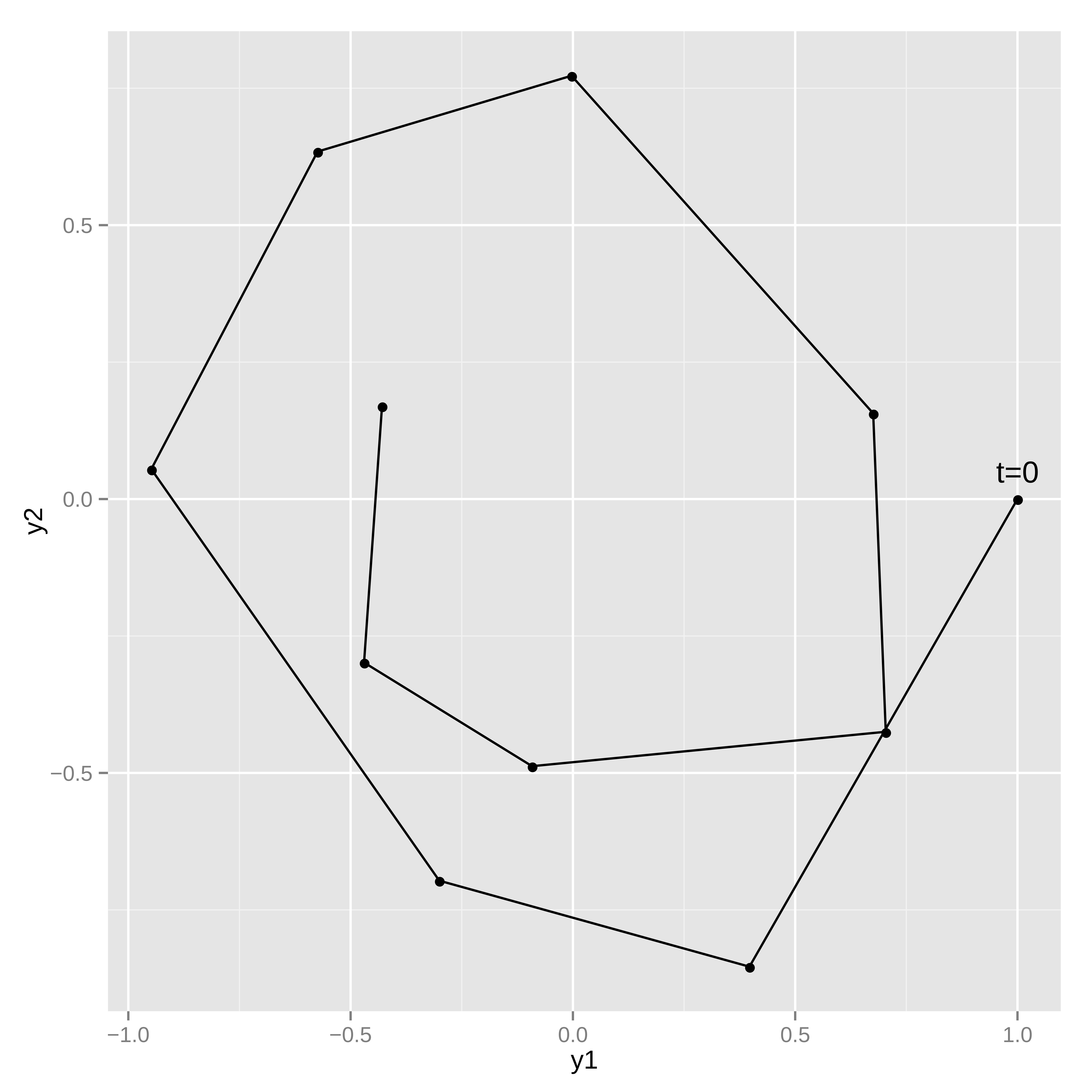
Figure 13.1: Typical realization of harmonic oscillator trajectory.

Estimating system parameters and initial state

These ten noisy observations of the state can be used to estimate the friction parameter, \(\theta\), the initial conditions, \(y(t_0, \theta)\), and the scale of the noise in the problem. The full Stan model is:

functions {
  vector sho(real t,
             vector y,
             real theta) {
    vector[2] dydt;
    dydt[1] = y[2];
    dydt[2] = -y[1] - theta * y[2];
    return dydt;
  }
}
data {
  int<lower=1> T;
  vector[2] y[T];
  real t0;
  real ts[T];
}
parameters {
  vector[2] y0;
  vector<lower=0>[2] sigma;
  real theta;
}
model {
  vector[2] mu[T] = ode_rk45(sho, y0, t0, ts, theta);
  sigma ~ normal(0, 2.5);
  theta ~ std_normal();
  y0 ~ std_normal();
  for (t in 1:T)
    y[t] ~ normal(mu[t], sigma);
}

Because the solves are now a function of model parameters, the ode_rk45 call is now made in the model block. There are half-normal priors on the measurement error scales sigma, and standard normal priors on theta and the initial state vector y0. The solutions to the ODE are assigned to mu, which is used as the location for the normal observation model.

As with other regression models, it’s easy to change the noise model to something with heavier tails (e.g., Student-t distributed), correlation in the state variables (e.g., with a multivariate normal distribution), or both heavy tails and correlation in the state variables (e.g., with a multivariate Student-t distribution).