PPC intervals

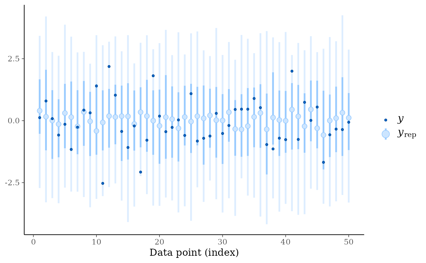
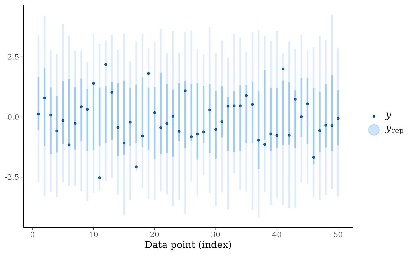
Medians and central interval estimates of yrep with y overlaid. See the Plot Descriptions section, below.

ppc_intervals(
  y,
  yrep,
  x = NULL,
  ...,
  prob = 0.5,
  prob_outer = 0.9,
  alpha = 0.33,
  size = 1,
  fatten = 2.5,
  linewidth = 1
)

ppc_intervals_grouped(
  y,
  yrep,
  x = NULL,
  group,
  ...,
  facet_args = list(),
  prob = 0.5,
  prob_outer = 0.9,
  alpha = 0.33,
  size = 1,
  fatten = 2.5,
  linewidth = 1
)

ppc_ribbon(
  y,
  yrep,
  x = NULL,
  ...,
  prob = 0.5,
  prob_outer = 0.9,
  alpha = 0.33,
  size = 0.25,
  y_draw = c("line", "points", "both")
)

ppc_ribbon_grouped(
  y,
  yrep,
  x = NULL,
  group,
  ...,
  facet_args = list(),
  prob = 0.5,
  prob_outer = 0.9,
  alpha = 0.33,
  size = 0.25,
  y_draw = c("line", "points", "both")
)

ppc_intervals_data(
  y,
  yrep,
  x = NULL,
  group = NULL,
  ...,
  prob = 0.5,
  prob_outer = 0.9
)

ppc_ribbon_data(
  y,
  yrep,
  x = NULL,
  group = NULL,
  ...,
  prob = 0.5,
  prob_outer = 0.9
)

Arguments

y

A vector of observations. See Details.

yrep

An S by N matrix of draws from the posterior (or prior) predictive distribution. The number of rows, S, is the size of the posterior (or prior) sample used to generate yrep. The number of columns, N is the number of predicted observations (length(y)). The columns of yrep should be in the same order as the data points in y for the plots to make sense. See the Details and Plot Descriptions sections for additional advice specific to particular plots.

x

A numeric vector to use as the x-axis variable. For example, x could be a predictor variable from a regression model, a time variable for time-series models, etc. If x is missing or NULL then the observation index is used for the x-axis.

...

Currently unused.

prob, prob_outer

Values between 0 and 1 indicating the desired probability mass to include in the inner and outer intervals. The defaults are prob=0.5 and prob_outer=0.9.

alpha, size, fatten, linewidth

Arguments passed to geoms. For ribbon plots alpha is passed to ggplot2::geom_ribbon() to control the opacity of the outer ribbon and size is passed to ggplot2::geom_line() to control the size of the line representing the median prediction (size=0 will remove the line). For interval plots alpha, size, fatten, and linewidth are passed to ggplot2::geom_pointrange() (fatten=0 will remove the point estimates).

group

A grouping variable of the same length as y. Will be coerced to factor if not already a factor. Each value in group is interpreted as the group level pertaining to the corresponding observation.

facet_args

A named list of arguments (other than facets) passed to ggplot2::facet_wrap() or ggplot2::facet_grid() to control faceting. Note: if scales is not included in facet_args then bayesplot may use scales="free" as the default (depending on the plot) instead of the ggplot2 default of scales="fixed".

y_draw

For ribbon plots only, a string specifying how to draw y. Can be "line" (the default), "points", or "both".

Value

The plotting functions return a ggplot object that can be further customized using the ggplot2 package. The functions with suffix _data() return the data that would have been drawn by the plotting function.

Plot Descriptions

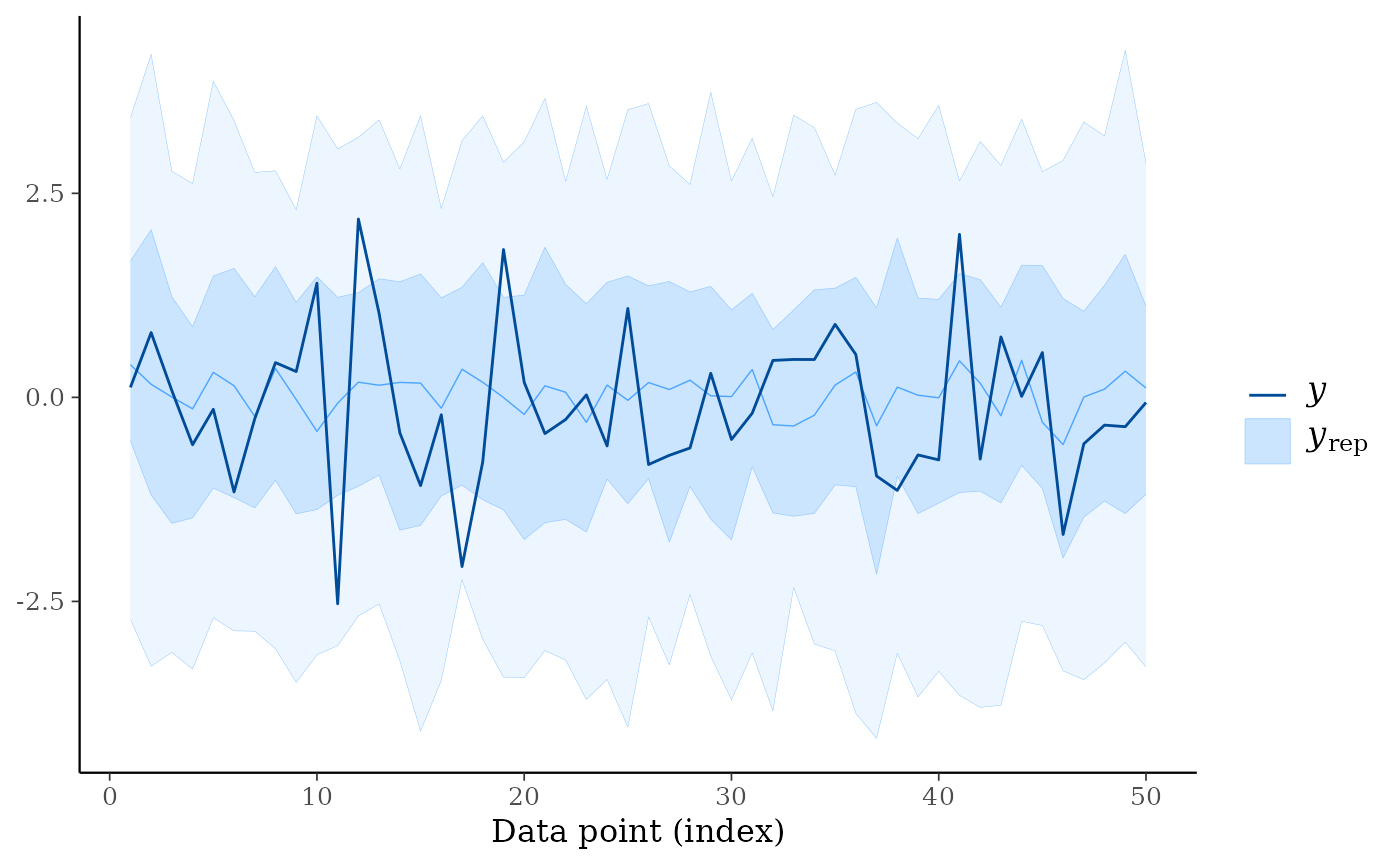
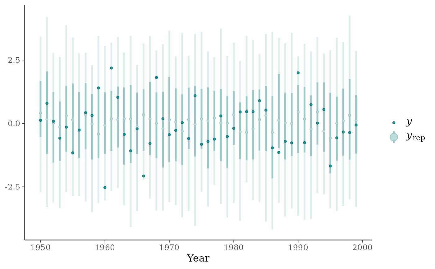
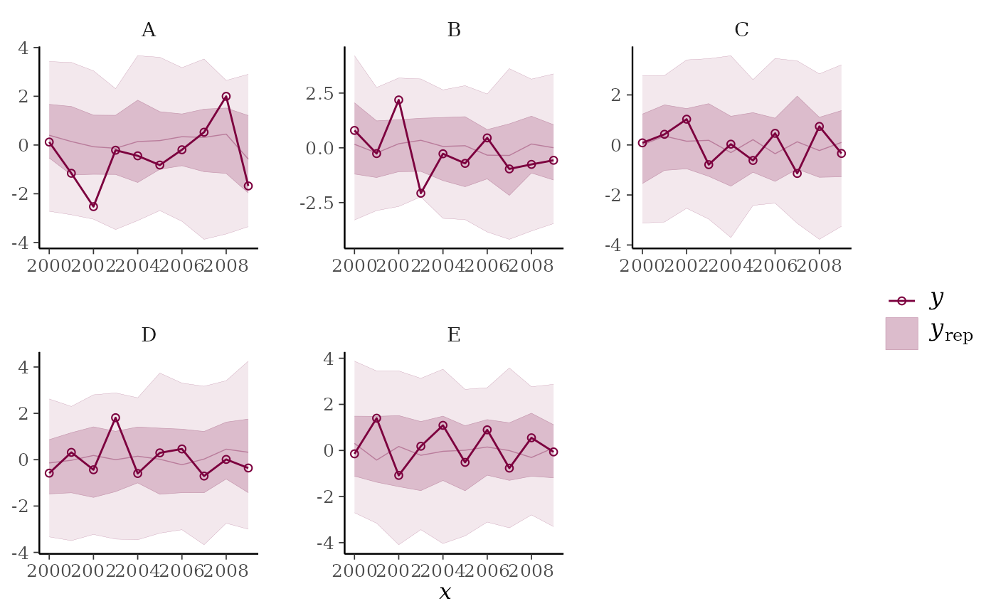
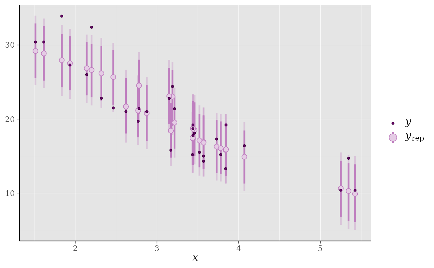
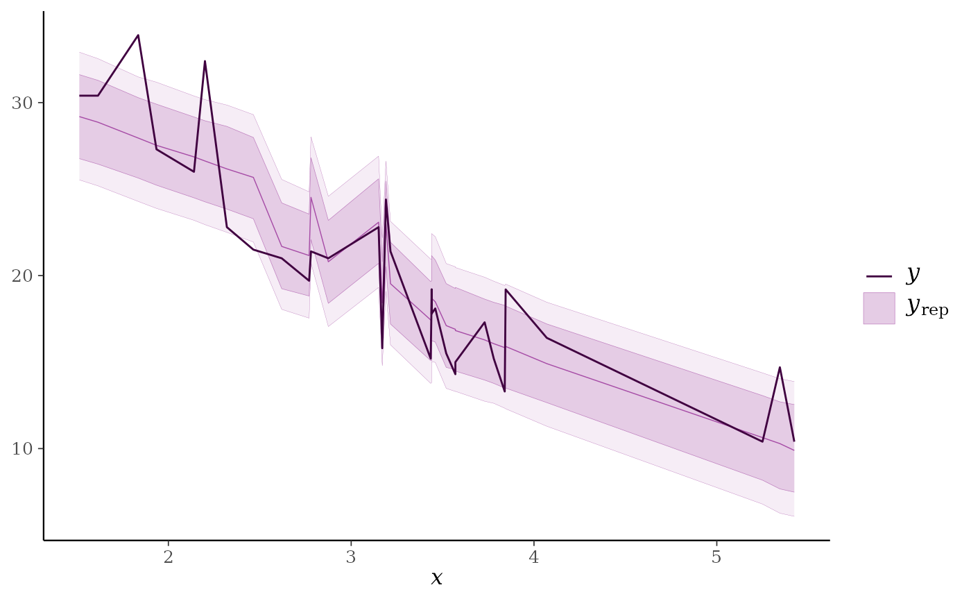
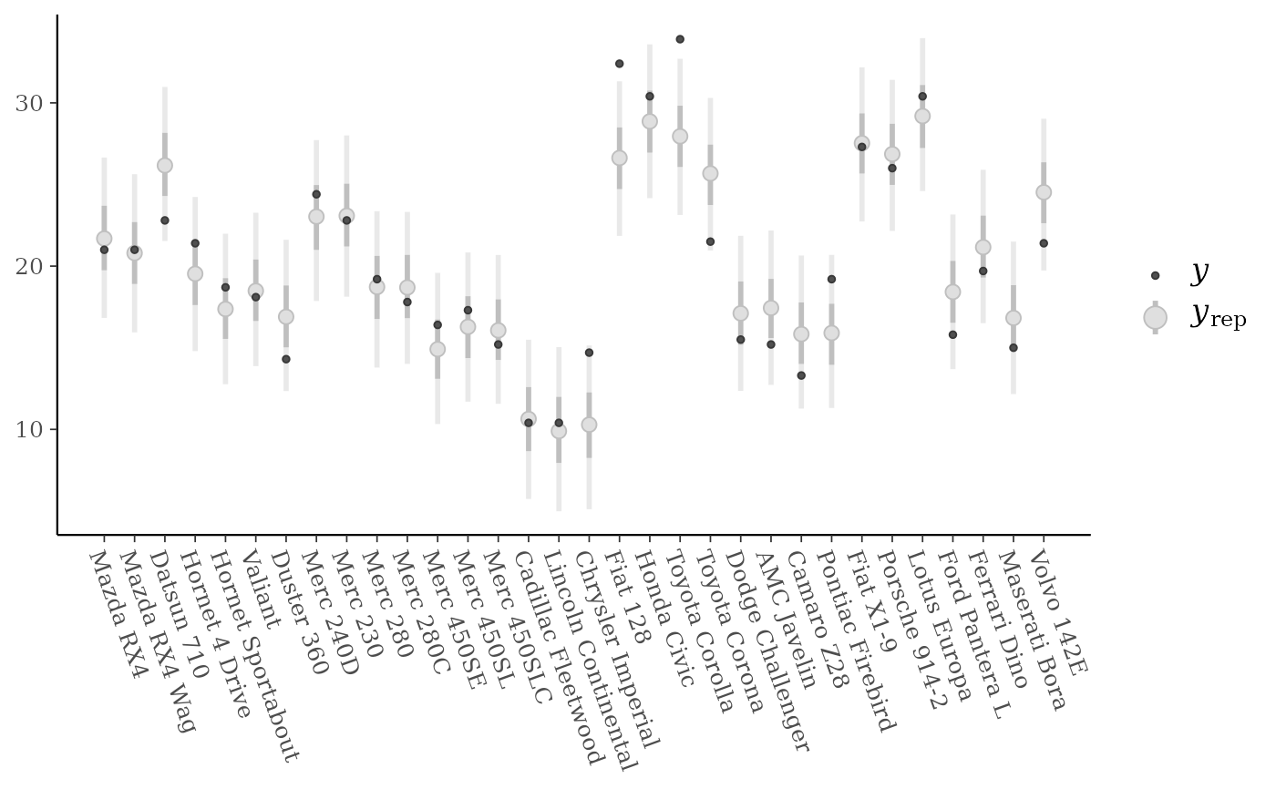
ppc_intervals(), ppc_ribbon()

100*prob% central intervals for yrep at each x value. ppc_intervals() plots intervals as vertical bars with points indicating yrep medians and darker points indicating observed y values. ppc_ribbon() plots a ribbon of connected intervals with a line through the median of yrep and a darker line connecting observed y values. In both cases an optional x variable can also be specified for the x-axis variable.

Depending on the number of observations and the variability in the predictions at different values of x, one of these plots may be easier to read than the other.

ppc_intervals_grouped(), ppc_ribbon_grouped()

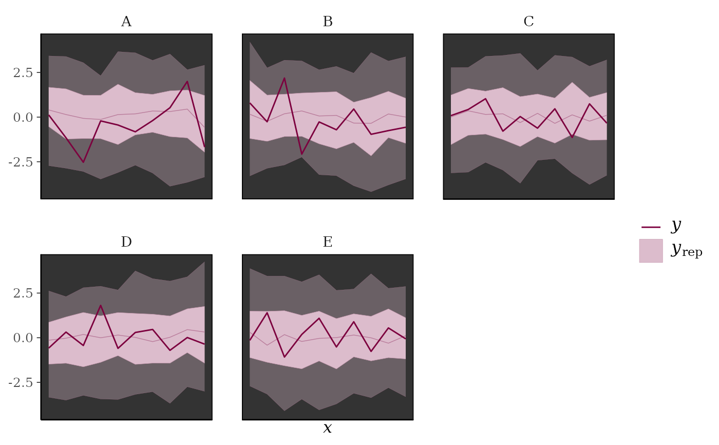
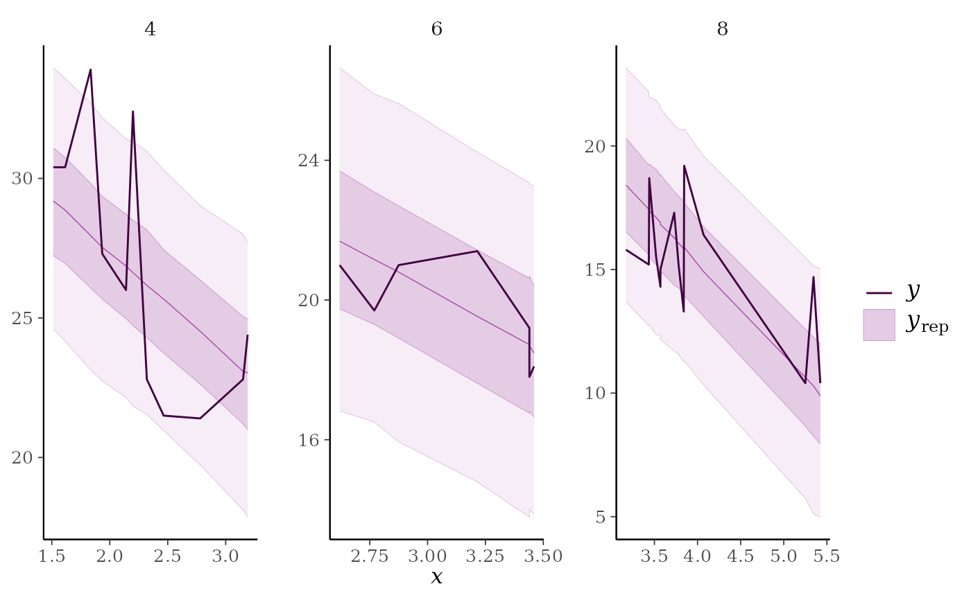
Same as ppc_intervals() and ppc_ribbon(), respectively, but a separate plot (facet) is generated for each level of a grouping variable.

References

Gabry, J. , Simpson, D. , Vehtari, A. , Betancourt, M. and Gelman, A. (2019), Visualization in Bayesian workflow. J. R. Stat. Soc. A, 182: 389-402. doi:10.1111/rssa.12378. (journal version, arXiv preprint, code on GitHub)

Gelman, A., Carlin, J. B., Stern, H. S., Dunson, D. B., Vehtari, A., and Rubin, D. B. (2013). Bayesian Data Analysis. Chapman & Hall/CRC Press, London, third edition. (Ch. 6)

See also

Other PPCs: PPC-censoring, PPC-discrete, PPC-distributions, PPC-errors, PPC-loo, PPC-overview, PPC-scatterplots, PPC-test-statistics

Examples

y <- rnorm(50)
yrep <- matrix(rnorm(5000, 0, 2), ncol = 50)

color_scheme_set("brightblue")
ppc_intervals(y, yrep)

ppc_ribbon(y, yrep)

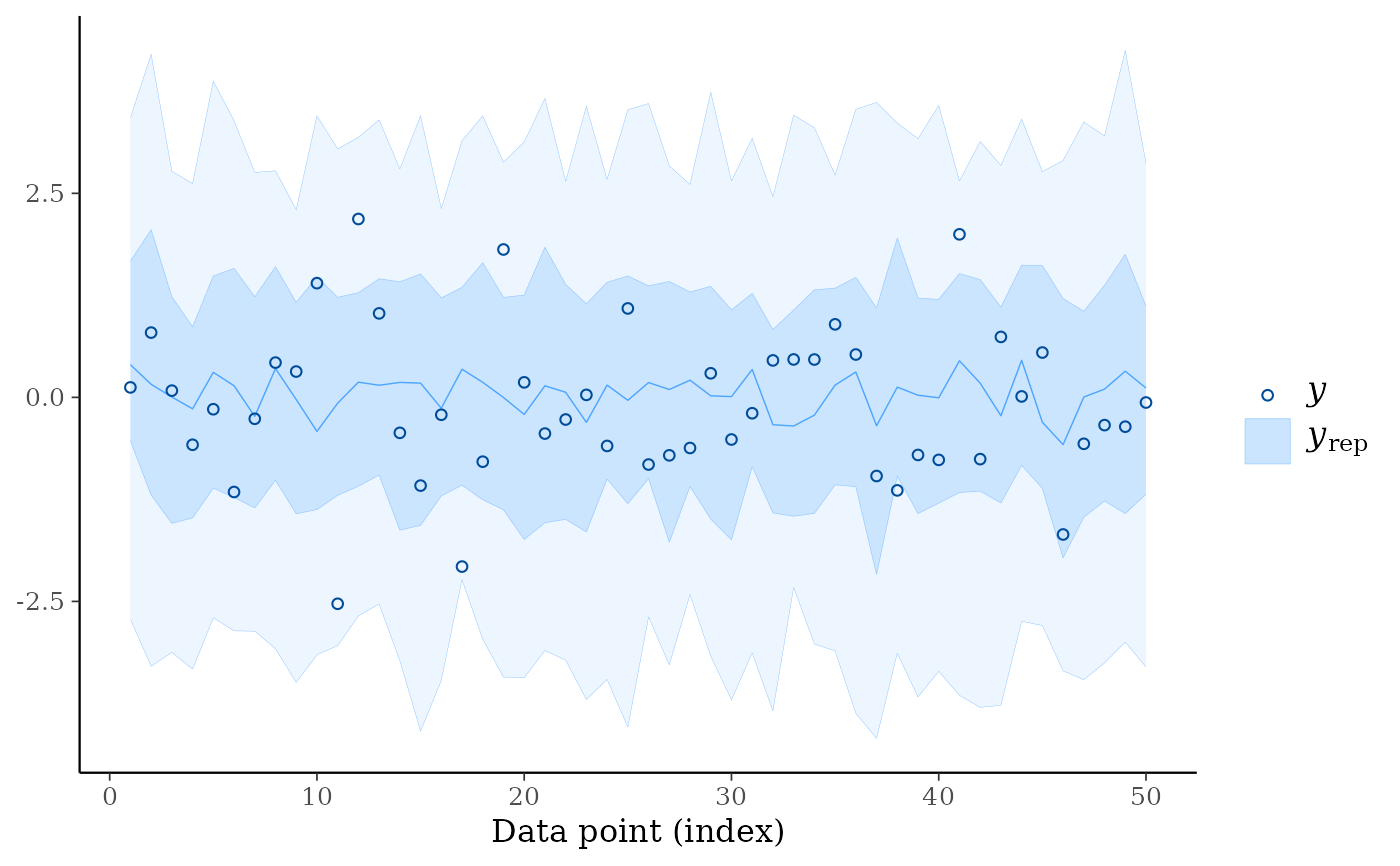
ppc_ribbon(y, yrep, y_draw = "points")

# \dontrun{
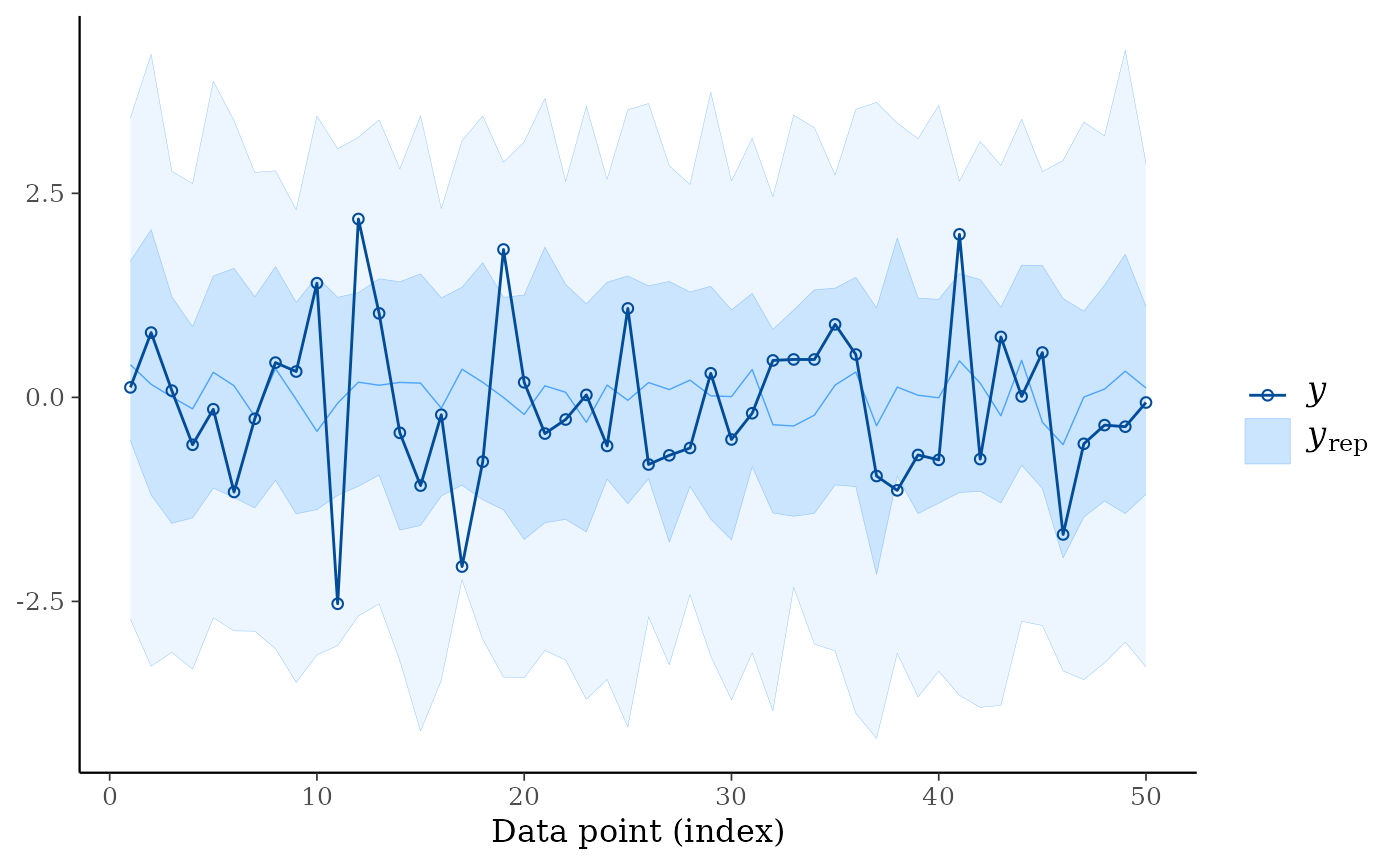
ppc_ribbon(y, yrep, y_draw = "both")

# }

ppc_intervals(y, yrep, size = 1.5, fatten = 0) # remove the yrep point estimates


color_scheme_set("teal")
year <- 1950:1999
ppc_intervals(y, yrep, x = year, fatten = 1) + ggplot2::xlab("Year")

ppc_ribbon(y, yrep, x = year) + ggplot2::xlab("Year")


color_scheme_set("pink")
year <- rep(2000:2009, each = 5)
group <- gl(5, 1, length = 50, labels = LETTERS[1:5])
ppc_ribbon_grouped(y, yrep, x = year, group, y_draw = "both") +
  ggplot2::scale_x_continuous(breaks = pretty)


ppc_ribbon_grouped(y, yrep, x = year, group,
                   facet_args = list(scales = "fixed")) +
 xaxis_text(FALSE) +
 xaxis_ticks(FALSE) +
 panel_bg(fill = "gray20")


# get the data frames used to make the ggplots
ppc_dat <- ppc_intervals_data(y, yrep, x = year, prob = 0.5)
ppc_group_dat <- ppc_intervals_data(y, yrep, x = year, group = group, prob = 0.5)

# \dontrun{
library("rstanarm")
fit <- stan_glmer(mpg ~ wt + (1|cyl), data = mtcars, refresh = 0)
yrep <- posterior_predict(fit)

color_scheme_set("purple")
ppc_intervals(y = mtcars$mpg, yrep = yrep, x = mtcars$wt, prob = 0.8) +
 panel_bg(fill="gray90", color = NA) +
 grid_lines(color = "white")


ppc_ribbon(y = mtcars$mpg, yrep = yrep, x = mtcars$wt,
           prob = 0.6, prob_outer = 0.8)


ppc_ribbon_grouped(y = mtcars$mpg, yrep = yrep, x = mtcars$wt,
                   group = mtcars$cyl)



color_scheme_set("gray")
ppc_intervals(mtcars$mpg, yrep, prob = 0.5) +
 ggplot2::scale_x_continuous(
   labels = rownames(mtcars),
   breaks = 1:nrow(mtcars)
 ) +
 xaxis_text(angle = -70, vjust = 1, hjust = 0) +
 xaxis_title(FALSE)


# }