Prior Distributions for rstanarm Models

Jonah Gabry and Ben Goodrich

2020-07-20

library(ggplot2)
library(bayesplot)
theme_set(bayesplot::theme_default())

July 2020 Update

As of July 2020 there are a few changes to prior distributions:

• Except for in default priors, autoscale now defaults to FALSE. This means that when specifying custom priors you no longer need to manually set autoscale=FALSE every time you use a distribution.

• There are minor changes to the default priors on the intercept and (non-hierarchical) regression coefficients. See Default priors and scale adjustments below.

We recommend the new book Regression and Other Stories, which discusses the background behind the default priors in rstanarm and also provides examples of specifying non-default priors.

Introduction

This vignette provides an overview of how the specification of prior distributions works in the rstanarm package. It is still a work in progress and more content will be added in future versions of rstanarm. Before reading this vignette it is important to first read the How to Use the rstanarm Package vignette, which provides a general overview of the package.

Every modeling function in rstanarm offers a subset of the arguments in the table below which are used for specifying prior distributions for the model parameters.

Argument	Used in	Applies to
prior_intercept	All modeling functions except stan_polr and stan_nlmer	Model intercept, after centering predictors.
prior	All modeling functions	Regression coefficients. Does not include coefficients that vary by group in a multilevel model (see prior_covariance).
prior_aux	stan_glm*, stan_glmer*, stan_gamm4, stan_nlmer	Auxiliary parameter, e.g. error SD (interpretation depends on the GLM).
prior_covariance	stan_glmer*, stan_gamm4, stan_nlmer	Covariance matrices in multilevel models with varying slopes and intercepts. See the stan_glmer vignette for details on this prior.

* stan_glm also implies stan_glm.nb. stan_glmer implies stan_lmer and stan_glmer.nb.

The stan_polr, stan_betareg, and stan_gamm4 functions also provide additional arguments specific only to those models:

Argument	Used only in	Applies to
prior_smooth	stan_gamm4	Prior for hyperparameters in GAMs (lower values yield less flexible smooth functions).
prior_counts	stan_polr	Prior counts of an ordinal outcome (when predictors at sample means).
prior_z	stan_betareg	Coefficients in the model for phi.
prior_intercept_z	stan_betareg	Intercept in the model for phi.
prior_phi	stan_betareg	phi, if not modeled as function of predictors.

To specify these arguments the user provides a call to one of the various available functions for specifying priors (e.g., prior = normal(0, 1), prior = cauchy(c(0, 1), c(1, 2.5))). The documentation for these functions can be found at help("priors"). The rstanarm documentation and the other vignettes provide many examples of using these arguments to specify priors and the documentation for these arguments on the help pages for the various rstanarm modeling functions (e.g., help("stan_glm")) also explains which distributions can be used when specifying each of the prior-related arguments.

Default (Weakly Informative) Prior Distributions

With very few exceptions, the default priors in rstanarm —the priors used if the arguments in the tables above are untouched— are not flat priors. Rather, the defaults are intended to be weakly informative. That is, they are designed to provide moderate regularization and help stabilize computation. For many (if not most) applications the defaults will perform well, but this is not guaranteed (there are no default priors that make sense for every possible model specification).

The way rstanarm attempts to make priors weakly informative by default is to internally adjust the scales of the priors. How this works (and, importantly, how to turn it off) is explained below, but first we can look at the default priors in action by fitting a basic linear regression model with the stan_glm function. For specifying priors, the stan_glm function accepts the arguments prior_intercept, prior, and prior_aux. To use the default priors we just leave those arguments at their defaults (i.e., we don’t specify them):

library("rstanarm")
default_prior_test <- stan_glm(mpg ~ wt + am, data = mtcars, chains = 1)

The prior_summary function provides a concise summary of the priors used:

prior_summary(default_prior_test)

Priors for model 'default_prior_test' 
------
Intercept (after predictors centered)
  Specified prior:
    ~ normal(location = 20, scale = 2.5)
  Adjusted prior:
    ~ normal(location = 20, scale = 15)

Coefficients
  Specified prior:
    ~ normal(location = [0,0], scale = [2.5,2.5])
  Adjusted prior:
    ~ normal(location = [0,0], scale = [15.40,30.20])

Auxiliary (sigma)
  Specified prior:
    ~ exponential(rate = 1)
  Adjusted prior:
    ~ exponential(rate = 0.17)
------
See help('prior_summary.stanreg') for more details

Starting from the bottom up, we can see that:

• Auxiliary: sigma, the error standard deviation, has a default prior that is \(\mathsf{exponential}(1)\). However, as a result of the automatic rescaling, the actual scale used was 6.03.

• Coefficients: By default the regression coefficients (in this case the coefficients on the wt and am variables) are treated as a priori independent with normal priors centered at 0 and with scale (standard deviation) \(2.5\). Like for sigma, in order for the default to be weakly informative rstanarm will adjust the scales of the priors on the coefficients. As a result, the prior scales actually used were 15.40 and 30.20.

• Intercept: For the intercept, the default prior is normal with mean \(0\) and standard deviation \(2.5\), but in this case the standard deviation was adjusted to 15.07. There is also a note in parentheses informing you that the prior applies to the intercept after all predictors have been centered (a similar note can be found in the documentation of the prior_intercept argument). In many cases the value of \(y\) when \(x=0\) is not meaningful and it is easier to think about the value when \(x = \bar{x}\). Therefore placing a prior on the intercept after centering the predictors typically makes it easier to specify a reasonable prior for the intercept. (Note: the user does not need to manually center the predictors.)

To disable the centering of the predictors, you need to omit the intercept from the model formula and include a column of ones as a predictor (which cannot be named "(Intercept)" in the data.frame). Then you can specify a prior “coefficient” for the column of ones.

The next two subsections describe how the rescaling works and how to easily disable it if desired.

Default priors and scale adjustments

Automatic scale adjustments happen in two cases:

1. When the default priors are used.
2. When the user sets autoscale=TRUE when specifying their own prior (e.g., normal(0, 3, autoscale=TRUE)). See help("priors") for a list of distributions to see which have an autoscale argument.

Here we describe how the default priors work for the intercept, regression coefficients, and (if applicable) auxiliary parameters. Autoscaling when not using default priors works analogously (if autoscale=TRUE).

Assume we have outcome \(y\) and predictors \(x_1,\ldots,x_k\) and our model has linear predictor

\[ \alpha + \beta_1 x_1 + \dots + \beta_K x_K. \]

Regression coefficients

The default prior on regression coefficients \(\beta_k\) is

\[ \beta_k \sim \mathsf{Normal}(0, \, 2.5 \cdot s_y/s_x) \] where \(s_x = \text{sd}(x)\) and \[ s_y = \begin{cases} \text{sd}(y) & \text{if } \:\: {\tt family=gaussian(link)}, \\ 1 & \text{otherwise}. \end{cases} \]

This corresponds to prior = normal(0, 2.5, autoscale = TRUE) in rstanarm code.

Intercept

The intercept is assigned a prior indirectly. The prior_intercept argument refers to the intercept after all predictors have been centered (internally by rstanarm). That is, instead of placing the prior on the expected value of \(y\) when \(x=0\), we place a prior on the expected value of \(y\) when \(x = \bar{x}\). The default prior for this centered intercept, say \(\alpha_c\), is

\[ \alpha_c \sim \mathsf{Normal}(m_y, \, 2.5 \cdot s_y) \] where

\[ m_y = \begin{cases} \bar{y} & \text{if } \:\: {\tt family=gaussian(link="identity")}, \\ 0 & \text{otherwise} \end{cases} \] and \(s_y\) is the same as above (either 1 or \(\text{sd(y)}\)).

Auxiliary parameters

The default prior on the auxiliary parameter (residual standard deviation for Gaussian, shape for gamma, reciprocal dispersion for negative binomial, etc.) is an exponential distribution with rate \(1/s_y\)

\[ \text{aux} \sim \mathsf{Exponential}(1/s_y) \] where \(s_y\) is the same as above (either 1 or \(\text{sd(y)}\)).

This corresponds to prior_aux = exponential(1, autoscale=TRUE) in rstanarm code.

Note on data-based priors

Because the scaling is based on the scales of the predictors (and possibly the outcome) these are technically data-dependent priors. However, since these priors are quite wide (and in most cases rather conservative), the amount of information used is weak and mainly takes into account the order of magnitude of the variables. This enables rstanarm to offer defaults that are reasonable for many models.

Disabling prior scale adjustments

To disable automatic rescaling simply specify a prior other than the default. rstanarm versions up to and including version 2.19.3 used to require you to explicitly set the autoscale argument to FALSE, but now autoscaling only happens by default for the default priors. To use autoscaling with manually specified priors you have to set autoscale = TRUE. For example, this prior specification will not include any autoscaling:

test_no_autoscale <-
  update(
    default_prior_test,
    prior = normal(0, 5),
    prior_intercept = student_t(4, 0, 10),
    prior_aux = cauchy(0, 3)
  )

We can verify that the prior scales weren’t adjusted by checking prior_summary:

prior_summary(test_no_autoscale)

Priors for model 'test_no_autoscale' 
------
Intercept (after predictors centered)
 ~ student_t(df = 4, location = 0, scale = 10)

Coefficients
 ~ normal(location = [0,0], scale = [5,5])

Auxiliary (sigma)
 ~ half-cauchy(location = 0, scale = 3)
------
See help('prior_summary.stanreg') for more details

How to Specify Flat Priors (and why you typically shouldn’t)

Uninformative is usually unwarranted and unrealistic (flat is frequently frivolous and fictional)

When “non-informative” or “uninformative” is used in the context of prior distributions, it typically refers to a flat (uniform) distribution or a nearly flat distribution. Sometimes it may also be used to refer to the parameterization-invariant Jeffreys prior. Although rstanarm does not prevent you from using very diffuse or flat priors, unless the data is very strong it is wise to avoid them.

Rarely is it appropriate in any applied setting to use a prior that gives the same (or nearly the same) probability mass to values near zero as it gives values bigger than the age of the universe in nanoseconds. Even a much narrower prior than that, e.g., a normal distribution with \(\sigma = 500\), will tend to put much more probability mass on unreasonable parameter values than reasonable ones. In fact, using the prior \(\theta \sim \mathsf{Normal(\mu = 0, \sigma = 500)}\) implies some strange prior beliefs. For example, you believe a priori that \(P(|\theta| < 250) < P(|\theta| > 250)\), which can easily be verified by doing the calculation with the normal CDF

p <- 1 - 2 * pnorm(-250, mean = 0, sd = 500)
print(paste("Pr(-250 < theta < 250) =", round(p, 2)))

[1] "Pr(-250 < theta < 250) = 0.38"

or via approximation with Monte Carlo draws:

theta <- rnorm(1e5, mean = 0, sd = 500)
p_approx <- mean(abs(theta) < 250)
print(paste("Pr(-250 < theta < 250) =", round(p_approx, 2)))

[1] "Pr(-250 < theta < 250) = 0.38"

d <- data.frame(theta, clr = abs(theta) > 250)
library(ggplot2)
ggplot(d, aes(x = theta, fill = clr)) +
  geom_histogram(binwidth = 5, show.legend = FALSE) +
  scale_y_continuous(name = "", labels = NULL, expand = c(0,0)) +
  scale_x_continuous(name = expression(theta), breaks = c(-1000, -250, 250, 1000))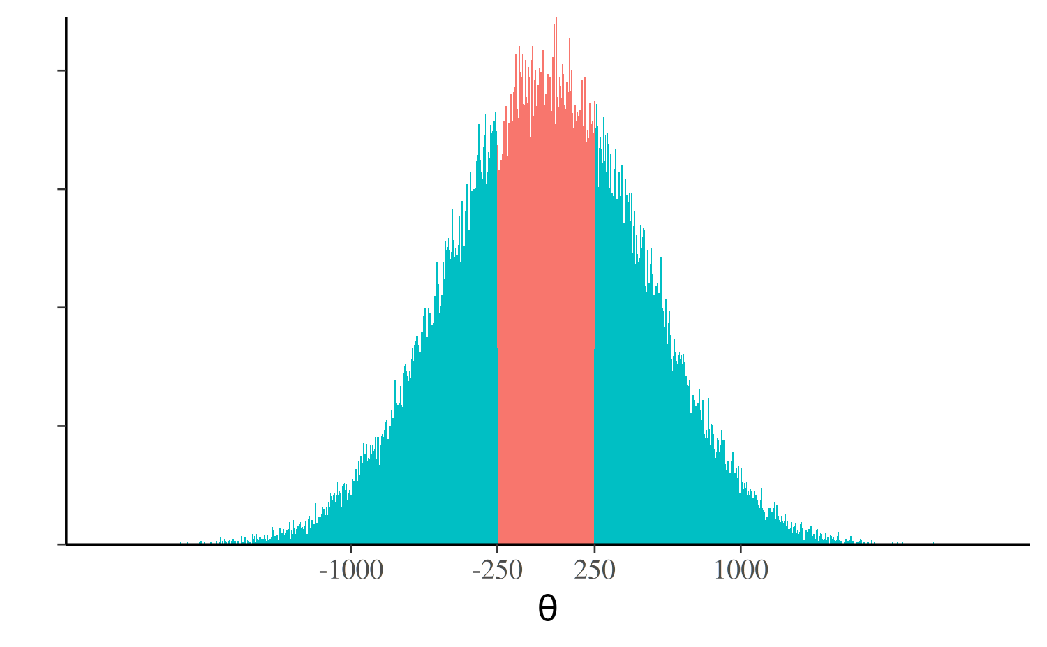

There is much more probability mass outside the interval (-250, 250).

This will almost never correspond to the prior beliefs of a researcher about a parameter in a well-specified applied regression model and yet priors like \(\theta \sim \mathsf{Normal(\mu = 0, \sigma = 500)}\) (and more extreme) remain quite popular.

Even when you know very little, a flat or very wide prior will almost never be the best approximation to your beliefs about the parameters in your model that you can express using rstanarm (or other software). Some amount of prior information will be available. For example, even if there is nothing to suggest a priori that a particular coefficient will be positive or negative, there is almost always enough information to suggest that different orders of magnitude are not equally likely. Making use of this information when setting a prior scale parameter is simple —one heuristic is to set the scale an order of magnitude bigger than you suspect it to be— and has the added benefit of helping to stabilize computations.

A more in-depth discussion of non-informative vs weakly informative priors is available in the case study How the Shape of a Weakly Informative Prior Affects Inferences.

Specifying flat priors

rstanarm will use flat priors if NULL is specified rather than a distribution. For example, to use a flat prior on regression coefficients you would specify prior=NULL:

flat_prior_test <- stan_glm(mpg ~ wt, data = mtcars, prior = NULL)

SAMPLING FOR MODEL 'continuous' NOW (CHAIN 1).
Chain 1: 
Chain 1: Gradient evaluation took 2.1e-05 seconds
Chain 1: 1000 transitions using 10 leapfrog steps per transition would take 0.21 seconds.
Chain 1: Adjust your expectations accordingly!
Chain 1: 
Chain 1: 
Chain 1: Iteration:    1 / 2000 [  0%]  (Warmup)
Chain 1: Iteration:  200 / 2000 [ 10%]  (Warmup)
Chain 1: Iteration:  400 / 2000 [ 20%]  (Warmup)
Chain 1: Iteration:  600 / 2000 [ 30%]  (Warmup)
Chain 1: Iteration:  800 / 2000 [ 40%]  (Warmup)
Chain 1: Iteration: 1000 / 2000 [ 50%]  (Warmup)
Chain 1: Iteration: 1001 / 2000 [ 50%]  (Sampling)
Chain 1: Iteration: 1200 / 2000 [ 60%]  (Sampling)
Chain 1: Iteration: 1400 / 2000 [ 70%]  (Sampling)
Chain 1: Iteration: 1600 / 2000 [ 80%]  (Sampling)
Chain 1: Iteration: 1800 / 2000 [ 90%]  (Sampling)
Chain 1: Iteration: 2000 / 2000 [100%]  (Sampling)
Chain 1: 
Chain 1:  Elapsed Time: 0.0423 seconds (Warm-up)
Chain 1:                0.040305 seconds (Sampling)
Chain 1:                0.082605 seconds (Total)
Chain 1: 

SAMPLING FOR MODEL 'continuous' NOW (CHAIN 2).
Chain 2: 
Chain 2: Gradient evaluation took 1.4e-05 seconds
Chain 2: 1000 transitions using 10 leapfrog steps per transition would take 0.14 seconds.
Chain 2: Adjust your expectations accordingly!
Chain 2: 
Chain 2: 
Chain 2: Iteration:    1 / 2000 [  0%]  (Warmup)
Chain 2: Iteration:  200 / 2000 [ 10%]  (Warmup)
Chain 2: Iteration:  400 / 2000 [ 20%]  (Warmup)
Chain 2: Iteration:  600 / 2000 [ 30%]  (Warmup)
Chain 2: Iteration:  800 / 2000 [ 40%]  (Warmup)
Chain 2: Iteration: 1000 / 2000 [ 50%]  (Warmup)
Chain 2: Iteration: 1001 / 2000 [ 50%]  (Sampling)
Chain 2: Iteration: 1200 / 2000 [ 60%]  (Sampling)
Chain 2: Iteration: 1400 / 2000 [ 70%]  (Sampling)
Chain 2: Iteration: 1600 / 2000 [ 80%]  (Sampling)
Chain 2: Iteration: 1800 / 2000 [ 90%]  (Sampling)
Chain 2: Iteration: 2000 / 2000 [100%]  (Sampling)
Chain 2: 
Chain 2:  Elapsed Time: 0.036959 seconds (Warm-up)
Chain 2:                0.039121 seconds (Sampling)
Chain 2:                0.07608 seconds (Total)
Chain 2: 

SAMPLING FOR MODEL 'continuous' NOW (CHAIN 3).
Chain 3: 
Chain 3: Gradient evaluation took 1.2e-05 seconds
Chain 3: 1000 transitions using 10 leapfrog steps per transition would take 0.12 seconds.
Chain 3: Adjust your expectations accordingly!
Chain 3: 
Chain 3: 
Chain 3: Iteration:    1 / 2000 [  0%]  (Warmup)
Chain 3: Iteration:  200 / 2000 [ 10%]  (Warmup)
Chain 3: Iteration:  400 / 2000 [ 20%]  (Warmup)
Chain 3: Iteration:  600 / 2000 [ 30%]  (Warmup)
Chain 3: Iteration:  800 / 2000 [ 40%]  (Warmup)
Chain 3: Iteration: 1000 / 2000 [ 50%]  (Warmup)
Chain 3: Iteration: 1001 / 2000 [ 50%]  (Sampling)
Chain 3: Iteration: 1200 / 2000 [ 60%]  (Sampling)
Chain 3: Iteration: 1400 / 2000 [ 70%]  (Sampling)
Chain 3: Iteration: 1600 / 2000 [ 80%]  (Sampling)
Chain 3: Iteration: 1800 / 2000 [ 90%]  (Sampling)
Chain 3: Iteration: 2000 / 2000 [100%]  (Sampling)
Chain 3: 
Chain 3:  Elapsed Time: 0.038547 seconds (Warm-up)
Chain 3:                0.039273 seconds (Sampling)
Chain 3:                0.07782 seconds (Total)
Chain 3: 

SAMPLING FOR MODEL 'continuous' NOW (CHAIN 4).
Chain 4: 
Chain 4: Gradient evaluation took 1.5e-05 seconds
Chain 4: 1000 transitions using 10 leapfrog steps per transition would take 0.15 seconds.
Chain 4: Adjust your expectations accordingly!
Chain 4: 
Chain 4: 
Chain 4: Iteration:    1 / 2000 [  0%]  (Warmup)
Chain 4: Iteration:  200 / 2000 [ 10%]  (Warmup)
Chain 4: Iteration:  400 / 2000 [ 20%]  (Warmup)
Chain 4: Iteration:  600 / 2000 [ 30%]  (Warmup)
Chain 4: Iteration:  800 / 2000 [ 40%]  (Warmup)
Chain 4: Iteration: 1000 / 2000 [ 50%]  (Warmup)
Chain 4: Iteration: 1001 / 2000 [ 50%]  (Sampling)
Chain 4: Iteration: 1200 / 2000 [ 60%]  (Sampling)
Chain 4: Iteration: 1400 / 2000 [ 70%]  (Sampling)
Chain 4: Iteration: 1600 / 2000 [ 80%]  (Sampling)
Chain 4: Iteration: 1800 / 2000 [ 90%]  (Sampling)
Chain 4: Iteration: 2000 / 2000 [100%]  (Sampling)
Chain 4: 
Chain 4:  Elapsed Time: 0.035293 seconds (Warm-up)
Chain 4:                0.02856 seconds (Sampling)
Chain 4:                0.063853 seconds (Total)
Chain 4: 

In this case we let rstanarm use the default priors for the intercept and error standard deviation (we could change that if we wanted), but the coefficient on the wt variable will have a flat prior. To double check that indeed a flat prior was used for the coefficient on wt we can call prior_summary:

prior_summary(flat_prior_test)

Priors for model 'flat_prior_test' 
------
Intercept (after predictors centered)
  Specified prior:
    ~ normal(location = 20, scale = 2.5)
  Adjusted prior:
    ~ normal(location = 20, scale = 15)

Coefficients
 ~ flat

Auxiliary (sigma)
  Specified prior:
    ~ exponential(rate = 1)
  Adjusted prior:
    ~ exponential(rate = 0.17)
------
See help('prior_summary.stanreg') for more details

Informative Prior Distributions

Although the default priors tend to work well, prudent use of more informative priors is encouraged. For example, suppose we have a linear regression model \[y_i \sim \mathsf{Normal}\left(\alpha + \beta_1 x_{1,i} + \beta_2 x_{2,i}, \, \sigma\right)\] and we have evidence (perhaps from previous research on the same topic) that approximately \(\beta_1 \in (-15, -5)\) and \(\beta_2 \in (-1, 1)\). An example of an informative prior for \(\boldsymbol{\beta} = (\beta_1, \beta_2)'\) could be

\[ \boldsymbol{\beta} \sim \mathsf{Normal} \left( \begin{pmatrix} -10 \\ 0 \end{pmatrix}, \begin{pmatrix} 5^2 & 0 \\ 0 & 2^2 \end{pmatrix} \right), \] which sets the prior means at the midpoints of the intervals and then allows for some wiggle room on either side. If the data are highly informative about the parameter values (enough to overwhelm the prior) then this prior will yield similar results to a non-informative prior. But as the amount of data and/or the signal-to-noise ratio decrease, using a more informative prior becomes increasingly important.

If the variables y, x1, and x2 are in the data frame dat then this model can be specified as

my_prior <- normal(location = c(-10, 0), scale = c(5, 2))
stan_glm(y ~ x1 + x2, data = dat, prior = my_prior)

We left the priors for the intercept and error standard deviation at their defaults, but informative priors can be specified for those parameters in an analogous manner.