Extract projected parameter draws and coerce to draws_matrix (see package posterior)

These are the posterior::as_draws() and posterior::as_draws_matrix() methods for projection objects (returned by project(), possibly as elements of a list). They extract the projected parameter draws and return them as a draws_matrix. In case of different (i.e., nonconstant) weights for the projected draws, a draws_matrix allows for a safer handling of these weights (safer in contrast to the matrix returned by as.matrix.projection()), in particular by providing the natural input for posterior::resample_draws() (see section "Examples" below).

# S3 method for projection
as_draws_matrix(x, ...)

# S3 method for projection
as_draws(x, ...)

Arguments

x

An object of class projection (returned by project(), possibly as elements of a list).

...

Arguments passed to as.matrix.projection(), except for allow_nonconst_wdraws_prj.

Value

An \(S_{\mathrm{prj}} \times Q\)

draws_matrix (see posterior::draws_matrix()) of projected draws, with \(S_{\mathrm{prj}}\) denoting the number of projected draws and \(Q\) the number of parameters. If the projected draws have nonconstant weights, posterior::weight_draws() is applied internally.

Details

In case of the augmented-data projection for a multilevel submodel of a brms::categorical() reference model, the multilevel parameters (and therefore also their names) slightly differ from those in the brms reference model fit (see section "Augmented-data projection" in extend_family()'s documentation).

Examples

# Data:
dat_gauss <- data.frame(y = df_gaussian$y, df_gaussian$x)

# The `stanreg` fit which will be used as the reference model (with small
# values for `chains` and `iter`, but only for technical reasons in this
# example; this is not recommended in general):
fit <- rstanarm::stan_glm(
  y ~ X1 + X2 + X3 + X4 + X5, family = gaussian(), data = dat_gauss,
  QR = TRUE, chains = 2, iter = 500, refresh = 0, seed = 9876
)

# Projection onto an arbitrary combination of predictor terms (with a small
# value for `nclusters`, but only for illustrative purposes; this is not
# recommended in general):
prj <- project(fit, predictor_terms = c("X1", "X3", "X5"), nclusters = 5,
               seed = 9182, verbose = FALSE)

# Applying the posterior::as_draws_matrix() generic to the output of
# project() dispatches to the projpred::as_draws_matrix.projection()
# method:
prj_draws <- posterior::as_draws_matrix(prj)
#> Loading required namespace: testthat

# Resample the projected draws according to their weights:
set.seed(3456)
prj_draws_resampled <- posterior::resample_draws(prj_draws, ndraws = 1000)

# The values from the following two objects should be the same (in general,
# this only holds approximately):
print(proportions(table(rownames(prj_draws_resampled))))
#> 
#>     1     2     3     4     5 
#> 0.226 0.214 0.186 0.212 0.162 
print(weights(prj_draws))
#> [1] 0.226 0.214 0.186 0.212 0.162

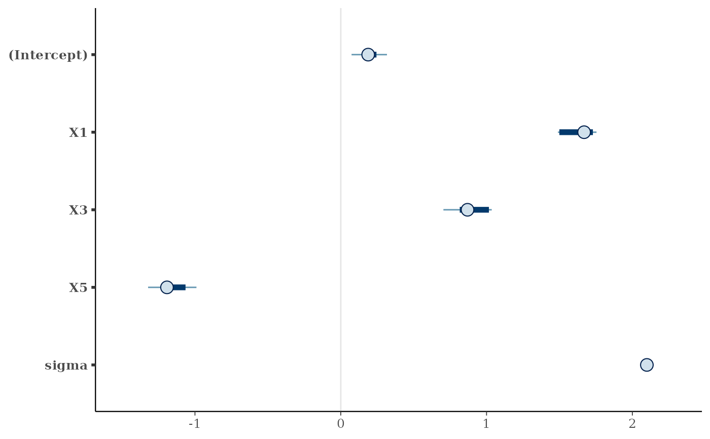
# Treat the resampled draws like ordinary draws, e.g., summarize them:
print(posterior::summarize_draws(
  prj_draws_resampled,
  "median", "mad", function(x) quantile(x, probs = c(0.025, 0.975))
))
#> # A tibble: 5 × 5
#>   variable    median    mad  `2.5%` `97.5%`
#>   <chr>        <dbl>  <dbl>   <dbl>   <dbl>
#> 1 (Intercept)  0.188 0.0841  0.0742   0.317
#> 2 X1           1.67  0.126   1.49     1.75 
#> 3 X3           0.869 0.218   0.704    1.04 
#> 4 X5          -1.19  0.189  -1.32    -0.990
#> 5 sigma        2.10  0.0185  2.09     2.12 
# Or visualize them using the `bayesplot` package:
if (requireNamespace("bayesplot", quietly = TRUE)) {
  print(bayesplot::mcmc_intervals(prj_draws_resampled))
}