Extract projected parameter draws and coerce to matrix

This is the as.matrix() method for projection objects (returned by project(), possibly as elements of a list). It extracts the projected parameter draws and returns them as a matrix. In case of different (i.e., nonconstant) weights for the projected draws, see as_draws_matrix.projection() for a better solution.

Usage

# S3 method for class 'projection'
as.matrix(x, nm_scheme = NULL, allow_nonconst_wdraws_prj = FALSE, ...)

Arguments

x

An object of class projection (returned by project(), possibly as elements of a list).

nm_scheme

The naming scheme for the columns of the output matrix. Either NULL, "rstanarm", or "brms", where NULL chooses "rstanarm" or "brms" based on the class of the reference model fit (and uses "rstanarm" if the reference model fit is of an unknown class).

allow_nonconst_wdraws_prj

A single logical value indicating whether to allow projected draws with different (i.e., nonconstant) weights (TRUE) or not (FALSE). CAUTION: Expert use only because if set to TRUE, the weights of the projected draws are stored in an attribute wdraws_prj and handling this attribute requires special care (e.g., when subsetting the returned matrix).

...

Currently ignored.

Value

An \(S_{\mathrm{prj}} \times Q\) matrix of projected draws, with \(S_{\mathrm{prj}}\) denoting the number of projected draws and \(Q\) the number of parameters. If allow_nonconst_wdraws_prj is set to TRUE, the weights of the projected draws are stored in an attribute wdraws_prj. (If allow_nonconst_wdraws_prj is FALSE, projected draws with nonconstant weights cause an error.)

Details

In case of the augmented-data projection for a multilevel submodel of a brms::categorical() reference model, the multilevel parameters (and therefore also their names) slightly differ from those in the brms reference model fit (see section "Augmented-data projection" in extend_family()'s documentation).

Examples

# Data:
dat_gauss <- data.frame(y = df_gaussian$y, df_gaussian$x)

# The `stanreg` fit which will be used as the reference model (with small
# values for `chains` and `iter`, but only for technical reasons in this
# example; this is not recommended in general):
fit <- rstanarm::stan_glm(
  y ~ X1 + X2 + X3 + X4 + X5, family = gaussian(), data = dat_gauss,
  QR = TRUE, chains = 2, iter = 500, refresh = 0, seed = 9876
)

# Projection onto an arbitrary combination of predictor terms (with a small
# value for `ndraws`, but only for the sake of speed in this example; this
# is not recommended in general):
prj <- project(fit, predictor_terms = c("X1", "X3", "X5"), ndraws = 21,
               seed = 9182)

# Applying the as.matrix() generic to the output of project() dispatches to
# the projpred::as.matrix.projection() method:
prj_mat <- as.matrix(prj)

# Since the draws have all the same weight here, we can treat them like
# ordinary MCMC draws, e.g., we can summarize them using the `posterior`
# package:
if (requireNamespace("posterior", quietly = TRUE)) {
  print(posterior::summarize_draws(
    posterior::as_draws_matrix(prj_mat),
    "median", "mad", function(x) quantile(x, probs = c(0.025, 0.975))
  ))
}
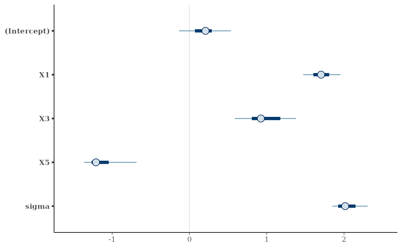
#> # A tibble: 5 × 5
#>   variable    median   mad `2.5%` `97.5%`
#>   <chr>        <dbl> <dbl>  <dbl>   <dbl>
#> 1 (Intercept)  0.207 0.202 -0.269   0.594
#> 2 X1           1.70  0.155  1.40    1.97 
#> 3 X3           0.924 0.266  0.560   1.45 
#> 4 X5          -1.21  0.111 -1.53   -0.602
#> 5 sigma        2.01  0.183  1.83    2.35 
# Or visualize them using the `bayesplot` package:
if (requireNamespace("bayesplot", quietly = TRUE)) {
  print(bayesplot::mcmc_intervals(prj_mat))
}