Plot method for stanreg objects

The plot method for stanreg-objects provides a convenient interface to the MCMC module in the bayesplot package for plotting MCMC draws and diagnostics. It is also straightforward to use the functions from the bayesplot package directly rather than via the plot method. Examples of both methods of plotting are given below.

Usage

# S3 method for class 'stanreg'
plot(x, plotfun = "intervals", pars = NULL, regex_pars = NULL, ...)

Arguments

x: A fitted model object returned by one of the rstanarm modeling functions. See stanreg-objects.
plotfun: A character string naming the bayesplot MCMC function to use. The default is to call mcmc_intervals. plotfun can be specified either as the full name of a bayesplot plotting function (e.g. "mcmc_hist") or can be abbreviated to the part of the name following the "mcmc_" prefix (e.g. "hist"). To get the names of all available MCMC functions see available_mcmc.
pars: An optional character vector of parameter names.
regex_pars: An optional character vector of regular expressions to use for parameter selection. regex_pars can be used in place of pars or in addition to pars. Currently, all functions that accept a regex_pars argument ignore it for models fit using optimization.
...: Additional arguments to pass to plotfun for customizing the plot. These are described on the help pages for the individual plotting functions. For example, the arguments accepted for the default plotfun="intervals" can be found at mcmc_intervals.

Value

Either a ggplot object that can be further customized using the ggplot2 package, or an object created from multiple ggplot objects (e.g. a gtable object created by arrangeGrob).

References

Gabry, J. , Simpson, D. , Vehtari, A. , Betancourt, M. and Gelman, A. (2019), Visualization in Bayesian workflow. J. R. Stat. Soc. A, 182: 389-402. doi:10.1111/rssa.12378, arXiv preprint, code on GitHub)

Examples

if (.Platform$OS.type != "windows" || .Platform$r_arch != "i386") {
# \donttest{
# Use rstanarm example model
if (!exists("example_model")) example(example_model)
fit <- example_model

#####################################
### Intervals and point estimates ###
#####################################
plot(fit) # same as plot(fit, "intervals"), plot(fit, "mcmc_intervals")

p <- plot(fit, pars = "size", regex_pars = "period",
          prob = 0.5, prob_outer = 0.9)
p + ggplot2::ggtitle("Posterior medians \n with 50% and 90% intervals")

# Shaded areas under densities
bayesplot::color_scheme_set("brightblue")
plot(fit, "areas", regex_pars = "period",
     prob = 0.5, prob_outer = 0.9)

# Make the same plot by extracting posterior draws and calling
# bayesplot::mcmc_areas directly
x <- as.array(fit, regex_pars = "period")
bayesplot::mcmc_areas(x, prob = 0.5, prob_outer = 0.9)

# Ridgelines version of the areas plot
bayesplot::mcmc_areas_ridges(x, regex_pars = "period", prob = 0.9)


##################################
### Histograms & density plots ###
##################################
plot_title <- ggplot2::ggtitle("Posterior Distributions")
plot(fit, "hist", regex_pars = "period") + plot_title
plot(fit, "dens_overlay", pars = "(Intercept)",
     regex_pars = "period") + plot_title

####################
### Scatterplots ###
####################
bayesplot::color_scheme_set("teal")
plot(fit, "scatter", pars = paste0("period", 2:3))
plot(fit, "scatter", pars = c("(Intercept)", "size"),
     size = 3, alpha = 0.5) +
     ggplot2::stat_ellipse(level = 0.9)


####################################################
### Rhat, effective sample size, autocorrelation ###
####################################################
bayesplot::color_scheme_set("red")

# rhat
plot(fit, "rhat")
plot(fit, "rhat_hist")

# ratio of effective sample size to total posterior sample size
plot(fit, "neff")
plot(fit, "neff_hist")

# autocorrelation by chain
plot(fit, "acf", pars = "(Intercept)", regex_pars = "period")
plot(fit, "acf_bar", pars = "(Intercept)", regex_pars = "period")


##################
### Traceplots ###
##################
# NOTE: rstanarm doesn't store the warmup draws (to save space because they
# are not so essential for diagnosing the particular models implemented in
# rstanarm) so the iterations in the traceplot are post-warmup iterations

bayesplot::color_scheme_set("pink")
(trace <- plot(fit, "trace", pars = "(Intercept)"))

# change traceplot colors to ggplot defaults or custom values
trace + ggplot2::scale_color_discrete()
trace + ggplot2::scale_color_manual(values = c("maroon", "skyblue2"))

# changing facet layout 
plot(fit, "trace", pars = c("(Intercept)", "period2"),
     facet_args = list(nrow = 2))
# same plot by calling bayesplot::mcmc_trace directly
x <- as.array(fit, pars = c("(Intercept)", "period2"))
bayesplot::mcmc_trace(x, facet_args = list(nrow = 2))


############
### More ###
############

# regex_pars examples
plot(fit, regex_pars = "herd:1\\]")
plot(fit, regex_pars = "herd:[279]")
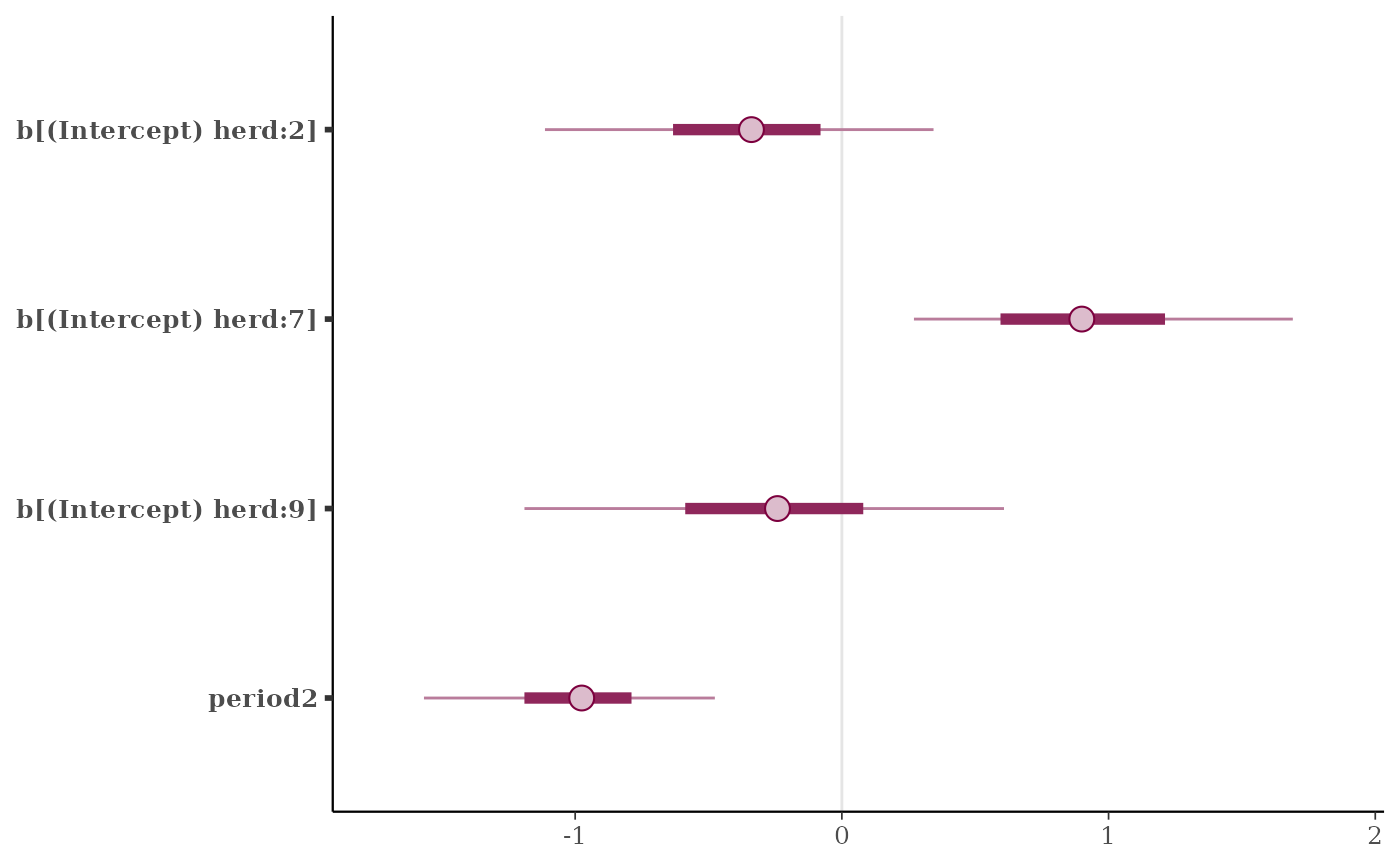
plot(fit, regex_pars = "herd:[279]|period2")
plot(fit, regex_pars = c("herd:[279]", "period2"))
# }

# For graphical posterior predictive checks see
# help("pp_check.stanreg")
}
#> Scale for colour is already present.
#> Adding another scale for colour, which will replace the existing scale.
#> Scale for colour is already present.
#> Adding another scale for colour, which will replace the existing scale.

Usage

Arguments

Value

References

See also

Examples