Estimating Joint Models for Longitudinal and Time-to-Event Data with rstanarm
Sam Brilleman
2025-12-30
Source:vignettes/jm.Rmd
jm.RmdPreamble
This vignette provides an introduction to the stan_jm
modelling function in the rstanarm package. The
stan_jm function allows the user to estimate a shared
parameter joint model for longitudinal and time-to-event data under a
Bayesian framework.
Introduction
Joint modelling can be broadly defined as the simultaneous estimation of two or more statistical models which traditionally would have been separately estimated. When we refer to a shared parameter joint model for longitudinal and time-to-event data, we generally mean the joint estimation of: 1) a longitudinal mixed effects model which analyses patterns of change in an outcome variable that has been measured repeatedly over time (for example, a clinical biomarker) and 2) a survival or time-to-event model which analyses the time until an event of interest occurs (for example, death or disease progression). Joint estimation of these so-called “submodels” is achieved by assuming they are correlated via individual-specific parameters (i.e. individual-level random effects).
Over the last two decades the joint modelling of longitudinal and
time-to-event data has received a significant amount of attention [1-5].
Methodological developments in the area have been motivated by a growing
awareness of the benefits that a joint modelling approach can provide.
In clinical or epidemiological research it is common for a clinical
biomarker to be repeatedly measured over time on a given patient. In
addition, it is common for time-to-event data, such as the
patient-specific time from a defined origin (e.g. time of diagnosis of a
disease) until a terminating clinical event such as death or disease
progression to also be collected. The figure below shows observed
longitudinal measurements (i.e. observed “trajectories”) of log serum
bilirubin for a small sample of patients with primary biliary cirrhosis.
Solid lines are used for those patients who were still alive at the end
of follow up, while dashed lines are used for those patients who died.
From the plots, we can observe between-patient variation in the
longitudinal trajectories for log serum bilirubin, with some patients
showing an increase in the biomarker over time, others decreasing, and
some remaining stable. Moreover, there is variation between patients in
terms of the frequency and timing of the longitudinal
measurements.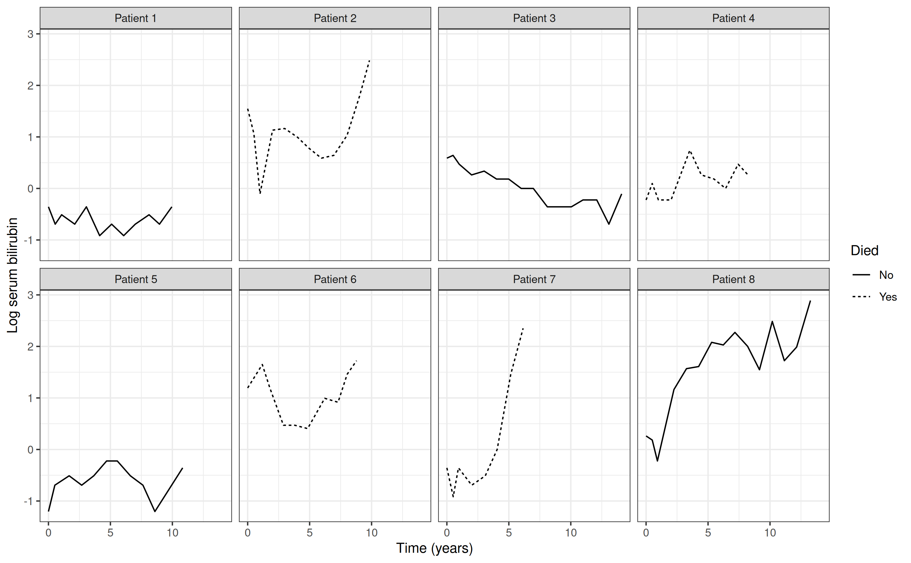
From the perspective of clinical risk prediction, we may be interested in asking whether the between-patient variation in the log serum bilirubin trajectories provides meaningful prognostic information that can help us differentiate patients with regard to some clinical event of interest, such as death. Alternatively, from an epidemiological perspective we may wish to explore the potential for etiological associations between changes in log serum bilirubin and mortality. Joint modelling approaches provide us with a framework under which we can begin to answer these types of clinical and epidemiological questions.
More formally, the motivations for undertaking a joint modelling analysis of longitudinal and time-to-event data might include one or more of the following:
One may be interested in how underlying changes in the biomarker influence the occurrence of the event. However, including the observed biomarker measurements directly into a time-to-event model as time-varying covariates poses several problems. For example, if the widely used Cox proportional hazards model is assumed for the time-to-event model then biomarker measurements need to be available for all patients at all failure times, which is unlikely to be the case [3]. If simple methods of imputation are used, such as the “last observation carried forward” method, then these are likely to induce bias [6]. Furthermore, the observed biomarker measurements may be subject to measurement error and therefore their inclusion as time-varying covariates may result in biased and inefficient estimates. In most cases, the measurement error will result in parameter estimates which are shrunk towards the null [7]. On the other hand, joint modelling approaches allow us to estimate the association between the biomarker (or some function of the biomarker trajectory, such as rate of change in the biomarker) and the risk of the event, whilst allowing for both the discrete time and measurement-error aspects of the observed biomarker.
One may be interested primarily in the evolution of the clinical biomarker but may wish to account for what is known as informative dropout. If the value of future (unobserved) biomarker measurements are related to the occurrence of the terminating event, then those unobserved biomarker measurements will be “missing not at random” [8,9]. In other words, biomarker measurements for patients who have an event will differ from those who do not have an event. Under these circumstances, inference based solely on observed measurements of the biomarker will be subject to bias. A joint modelling approach can help to adjust for informative dropout and has been shown to reduce bias in the estimated parameters associated with longitudinal changes in the biomarker [1,9,10].
Joint models are naturally suited to the task of dynamic risk prediction. For example, joint modelling approaches have been used to develop prognostic models where predictions of event risk can be updated as new longitudinal biomarker measurements become available. Taylor et al. [11] jointly modelled longitudinal measurements of the prostate specific antigen (PSA) and time to clinical recurrence of prostate cancer. The joint model was then used to develop a web-based calculator which could provide real-time predictions of the probability of recurrence based on a patient’s up to date PSA measurements.
In this vignette, we describe the rstanarm package’s
stan_jm modelling function. This modelling function allows
users to fit a shared parameter joint model for longitudinal and
time-to-event data under a Bayesian framework, with the backend
estimation carried out using Stan. In Section 2 we describe the
formulation of the joint model used by stan_jm. In Section
3 we present a variety of examples showing the usage of
stan_jm.
Note that some aspects of the estimation are covered in other vignettes, such as the priors vignette which contains details on the prior distributions available for regression coefficients.
Technical details
Model formulation
A shared parameter joint model consists of related submodels which are specified separately for each of the longitudinal and time-to-event outcomes. These are therefore commonly referred to as the longitudinal submodel(s) and the event submodel. The longitudinal and event submodels are linked using shared individual-specific parameters, which can be parameterised in a number of ways. We describe each of these submodels below.
Longitudinal submodel(s)
We assume \(y_{ijm}(t) = y_{im}(t_{ij})\) corresponds to the observed value of the \(m^{th}\) \((m = 1,...,M)\) biomarker for individual \(i\) \((i = 1,...,N)\) taken at time point \(t_{ij}\), \(j = 1,...,n_{im}\). We specify a (multivariate) generalised linear mixed model that assumes \(y_{ijm}(t)\) follows a distribution in the exponential family with mean \(\mu_{ijm}(t)\) and linear predictor
\[ \eta_{ijm}(t) = g_m(\mu_{ijm}(t)) = \boldsymbol{x}^T_{ijm}(t) \boldsymbol{\beta}_m + \boldsymbol{z}^T_{ijm}(t) \boldsymbol{b}_{im} \]
where \(\boldsymbol{x}^T_{ijm}(t)\) and \(\boldsymbol{z}^T_{ijm}(t)\) are both row-vectors of covariates (which likely include some function of time, for example a linear slope, cubic splines, or polynomial terms) with associated vectors of fixed and individual-specific parameters \(\boldsymbol{\beta}_m\) and \(\boldsymbol{b}_{im}\), respectively, and \(g_m\) is some known link function. The distribution and link function are allowed to differ over the \(M\) longitudinal submodels. We let the vector \(\boldsymbol{\beta} = \{ \boldsymbol{\beta}_m ; m = 1,...,M\}\) denote the collection of population-level parameters across the \(M\) longitudinal submodels. We assume that the dependence across the different longitudinal submodels (i.e. the correlation between the different longitudinal biomarkers) is captured through a shared multivariate normal distribution for the individual-specific parameters; that is, we assume
\[ \begin{pmatrix} \boldsymbol{b}_{i1} \\ \vdots \\ \boldsymbol{b}_{iM} \end{pmatrix} = \boldsymbol{b}_i \sim \mathsf{Normal} \left( 0 , \boldsymbol{\Sigma} \right) \]
for some unstructured variance-covariance matrix \(\boldsymbol{\Sigma}\).
Event submodel
We assume that we also observe an event time \(T_i = \mathsf{min} \left( T^*_i , C_i \right)\) where \(T^*_i\) denotes the so-called “true” event time for individual \(i\) (potentially unobserved) and \(C_i\) denotes the censoring time. We define an event indicator \(d_i = I(T^*_i \leq C_i)\). We then model the hazard of the event using a parametric proportional hazards regression model of the form
\[ h_i(t) = h_0(t; \boldsymbol{\omega}) \mathsf{exp} \left( \boldsymbol{w}^T_i(t) \boldsymbol{\gamma} + \sum_{m=1}^M \sum_{q=1}^{Q_m} f_{mq}(\boldsymbol{\beta}, \boldsymbol{b}_{i}, \alpha_{mq}; t) \right) \]
where \(h_i(t)\) is the hazard of the event for individual \(i\) at time \(t\), \(h_0(t; \boldsymbol{\omega})\) is the baseline hazard at time \(t\) given parameters \(\boldsymbol{\omega}\), \(\boldsymbol{w}^T_i(t)\) is a row-vector of individual-specific covariates (possibly time-dependent) with an associated vector of regression coefficients \(\boldsymbol{\gamma}\) (log hazard ratios), \(f_{mq}(.)\) are a set of known functions for \(m=1,...,M\) and \(q=1,...,Q_m\), and the \(\alpha_{mq}\) are regression coefficients (log hazard ratios).
The longitudinal and event submodels are assumed to be related via an “association structure”, which is a set of functions each \(\{ f_{mq} ; m = 1,...,M, q = 1,...,Q_m \}\) that may each be conditional on the population-level parameters from the longitudinal submodel \(\boldsymbol{\beta}\), the individual-specific parameters \(\boldsymbol{b}_{i}\), and the population-level parameters \(\alpha_{mq}\) for \(m=1,...,M\) and \(q=1,...,Q_m\). That is, the association structure of the joint model is captured via the \(\sum_{m=1}^M \sum_{q=1}^{Q_m} f_{mq}(\boldsymbol{\beta}_m, \boldsymbol{b}_{im}, \alpha_{mq}; t)\) term in the linear predictor of the event submodel. The \(\alpha_{mq}\) are referred to as the “association parameters” since they quantify the strength of the association between the longitudinal and event processes. The various ways in which the association structure can be are described in the next section.
The probability of individual \(i\) still being event-free at time \(t\), often referred to as the “survival probability”, is defined as
\[ S_i(t) = \text{Prob} \Big( T_i^* \geq t \Big) = \exp \Big( -H_i(t) \Big) \]
where \(H_i(t) = \int_{s=0}^t h_i(s) ds\) is the cumulative hazard for individual \(i\).
We assume that the baseline hazard \(h_0(t;
\boldsymbol{\omega})\) is modelled parametrically. In the
stan_jm modelling function the baseline hazard be specified
as either: an approximation using B-splines on the log hazard scale (the
default); a Weibull distribution; or an approximation using a piecewise
constant function on the log hazard scale (sometimes referred to as
piecewise exponential). The choice of baseline hazard can be made via
the basehaz argument. In the case of the B-splines or
piecewise constant baseline hazard, the user can control the flexibility
by specifying the knots or degrees of freedom via the
basehaz_ops argument. (Note that currently there is
slightly limited post-estimation functionality available for models
estimated with a piecewise constant baseline hazard, so this is perhaps
the least preferable choice).
Association structures
As mentioned in the previous section, the dependence between the longitudinal and event submodels is captured through the association structure, which can be specified in a number of ways. The simplest association structure is likely to be
\[ f_{mq}(\boldsymbol{\beta}, \boldsymbol{b}_{im}, \alpha_{mq}; t) = \alpha_{mq} \eta_{im}(t) \]
and this is often referred to as a current value association structure since it assumes that the log hazard of the event at time \(t\) is linearly associated with the value of the longitudinal submodel’s linear predictor also evaluated at time \(t\). This is the most common association structure used in the joint modelling literature to date. In the situation where the longitudinal submodel is based on an identity link function and normal error distribution (i.e. a linear mixed model) the current value association structure can be viewed as a method for including the underlying “true” value of the biomarker as a time-varying covariate in the event submodel.1
However, other association structures are also possible. For example, we could assume the log hazard of the event is linearly associated with the current slope (i.e. rate of change) of the longitudinal submodel’s linear predictor, that is
\[ f_{mq}(\boldsymbol{\beta}, \boldsymbol{b}_{i}, \alpha_{mq}; t) = \alpha_{mq} \frac{d\eta_{im}(t)}{dt} \]
There are in fact a whole range of possible association structures, many of which have been discussed in the literature [14-16].
The stan_jm modelling function in the
rstanarm package allows for the following association
structures, which are specified via the assoc argument:
Current value (of the linear predictor or expected value) \[ f_{mq}(\boldsymbol{\beta}, \boldsymbol{b}_{i}, \alpha_{mq}; t) = \alpha_{mq} \eta_{im}(t) \\ f_{mq}(\boldsymbol{\beta}, \boldsymbol{b}_{i}, \alpha_{mq}; t) = \alpha_{mq} \mu_{im}(t) \]
Current slope (of the linear predictor or expected value) \[ f_{mq}(\boldsymbol{\beta}, \boldsymbol{b}_{i}, \alpha_{mq}; t) = \alpha_{mq} \frac{d\eta_{im}(t)}{dt} \\ f_{mq}(\boldsymbol{\beta}, \boldsymbol{b}_{i}, \alpha_{mq}; t) = \alpha_{mq} \frac{d\mu_{im}(t)}{dt} \]
Area under the curve (of the linear predictor or expected value) \[ f_{mq}(\boldsymbol{\beta}, \boldsymbol{b}_{i}, \alpha_{mq}; t) = \alpha_{mq} \int_0^t \eta_{im}(u) du \\ f_{mq}(\boldsymbol{\beta}, \boldsymbol{b}_{i}, \alpha_{mq}; t) = \alpha_{mq} \int_0^t \mu_{im}(u) du \]
Interactions between different biomarkers \[ f_{mq}(\boldsymbol{\beta}, \boldsymbol{b}_{i}, \alpha_{mq}; t) = \alpha_{mq} \eta_{im}(t) \eta_{im'}(t) \text{ for some } m = m' \text{ or } m \neq m' \\ f_{mq}(\boldsymbol{\beta}, \boldsymbol{b}_{i}, \alpha_{mq}; t) = \alpha_{mq} \eta_{im}(t) \mu_{im'}(t) \text{ for some } m = m' \text{ or } m \neq m' \\ f_{mq}(\boldsymbol{\beta}, \boldsymbol{b}_{i}, \alpha_{mq}; t) = \alpha_{mq} \mu_{im}(t) \mu_{im'}(t) \text{ for some } m = m' \text{ or } m \neq m' \]
Interactions between the biomarker (or it’s slope) and observed data \[ f_{mq}(\boldsymbol{\beta}, \boldsymbol{b}_{i}, \alpha_{mq}; t) = \alpha_{mq} c_{i}(t) \eta_{im}(t) \text{ for some covariate value } c_{i}(t) \\ f_{mq}(\boldsymbol{\beta}, \boldsymbol{b}_{i}, \alpha_{mq}; t) = \alpha_{mq} c_{i}(t) \mu_{im}(t) \text{ for some covariate value } c_{i}(t) \\ f_{mq}(\boldsymbol{\beta}, \boldsymbol{b}_{i}, \alpha_{mq}; t) = \alpha_{mq} c_{i}(t) \frac{d\eta_{im}(t)}{dt} \text{ for some covariate value } c_{i}(t) \\ f_{mq}(\boldsymbol{\beta}, \boldsymbol{b}_{i}, \alpha_{mq}; t) = \alpha_{mq} c_{i}(t) \frac{d\mu_{im}(t)}{dt} \text{ for some covariate value } c_{i}(t) \]
As well as using lagged values for any of the above. That is, replacing \(t\) with \(t-u\) where \(u\) is some lag time, such that the hazard of the event at time \(t\) is assumed to be associated with some function of the longitudinal submodel parameters at time \(t-u\).
Lastly, we can specify some time-independent function of the random effects, possibly including the fixed effect component. For example,
\[ f_{mq}(\boldsymbol{\beta}, \boldsymbol{b}_{i}, \alpha_{mq}; t) = \alpha_{mq} \boldsymbol{b}_{im0} \]
or
\[ f_{mq}(\boldsymbol{\beta}, \boldsymbol{b}_{i}, \alpha_{mq}; t) = \alpha_{mq} \Big( \boldsymbol{\beta}_{m0} + \boldsymbol{b}_{im0} \Big) \]
where \(\boldsymbol{\beta}_{m0}\) is the population-level intercept for the \(m^{th}\) longitudinal submodel and \(\boldsymbol{b}_{im0}\) is the \(i^{th}\) individual’s random deviation from the population-level intercept for the \(m^{th}\) longitudinal submodel.
Note that more than one association structure can be specified,
however, not all possible combinations are allowed. Moreover, if you are
fitting a multivariate joint model (i.e. more than one longitudinal
outcome) then you can optionally choose to use a different association
structure(s) for linking each longitudinal submodel to the event
submodel. To do this you can pass a list of length \(M\) to the assoc argument.
Assumptions
Here we define a set of assumptions for the multivariate shared parameter joint model.
The so-called conditional independence assumption of the shared parameter joint model postulates
\[ y_{im}(t) \perp y_{im'}(t) \mid \boldsymbol{b}_i, \boldsymbol{\theta} \\ y_{im}(t) \perp y_{im}(t') \mid \boldsymbol{b}_i, \boldsymbol{\theta} \\ y_{im}(t) \perp T_i^* \mid \boldsymbol{b}_i, \boldsymbol{\theta} \]
for some \(m \neq m'\) and \(t \neq t'\), and where \(\boldsymbol{\theta}\) denotes the combined vector of all remaining population-level parameters in the model. That is, conditional on the individual-specific parameters \(\boldsymbol{b}_i\) and population-level parameters \(\boldsymbol{\theta}\), the following are assumed: (i) any biomarker measurement for individual \(i\) is independent of that individual’s true event time \(T_i^*\); (ii) any two measurements of the \(m^{th}\) biomarker taken on the \(i^{th}\) individual at two distinct time points \(t\) and \(t'\) (i.e. longitudinal or repeated measurements) are independent of one another; and (iii) any two measurements of two different biomarkers, taken on the \(i^{th}\) individual at some time point \(t\) are independent of one another. These conditional independence assumptions allow for a convenient factorisation of the full likelihood for joint model into the likelihoods for each of the component parts (i.e. the likelihood for the longitudinal submodel, the likelihood for the event submodel, and the likelihood for the distribution of the individual-specific parameters), which facilitates the estimation of the model.
Moreover, we require two additional assumptions: (i) that the censoring process for the event outcome is independent of the true event time, that is \(C_i \perp T_i^* \mid \boldsymbol{\theta}\) (i.e. uninformative censoring); and (ii) that the visiting process by which the observation times \(t_{ijm}\) are determined is independent of the true event time \(T_i^*\) and all missing future unobserved longitudinal biomarker measurements.
Log posterior distribution
Under the conditional independence assumption, the log posterior for the \(i^{th}\) individual can be specified as
\[ \log p(\boldsymbol{\theta}, \boldsymbol{b}_{i} \mid \boldsymbol{y}_{i}, T_i, d_i) \propto \log \Bigg[ \Bigg( \prod_{m=1}^M \prod_{j=1}^{n_i} p(y_{ijm}(t) \mid \boldsymbol{b}_{i}, \boldsymbol{\theta}) \Bigg) p(T_i, d_i \mid \boldsymbol{b}_{i}, \boldsymbol{\theta}) p(\boldsymbol{b}_{i} \mid \boldsymbol{\theta}) p(\boldsymbol{\theta}) \Bigg] \]
where \(\boldsymbol{y}_i = \{ y_{ijm}(t); j = 1,...,n_i, m = 1,...,M \}\) denotes the collection of longitudinal biomarker data for individual \(i\) and \(\boldsymbol{\theta}\) denotes all remaining population-level parameters in the model.
We can rewrite this log posterior as
\[ \log p(\boldsymbol{\theta}, \boldsymbol{b}_{i} \mid \boldsymbol{y}_{i}, T_i, d_i) \propto \Bigg( \sum_{m=1}^M \sum_{j=1}^{n_i} \log p(y_{ijm}(t) \mid \boldsymbol{b}_{i}, \boldsymbol{\theta}) \Bigg) + \log p(T_i, d_i \mid \boldsymbol{b}_{i}, \boldsymbol{\theta}) + \log p(\boldsymbol{b}_{i} \mid \boldsymbol{\theta}) + \log p(\boldsymbol{\theta}) \]
where \(\sum_{j=1}^{n_{im}} \log p(y_{ijm} \mid \boldsymbol{b}_{i}, \boldsymbol{\theta})\) is the log likelihood for the \(m^{th}\) longitudinal submodel, \(\log p(T_i, d_i \mid \boldsymbol{b}_{i}, \boldsymbol{\theta})\) is the log likelihood for the event submodel, \(\log p(\boldsymbol{b}_{i} \mid \boldsymbol{\theta})\) is the log likelihood for the distribution of the group-specific parameters (i.e. random effects), and \(\log p(\boldsymbol{\theta})\) represents the log likelihood for the joint prior distribution across all remaining unknown parameters.2
We can rewrite the log likelihood for the event submodel as
\[ \log p(T_i, d_i \mid \boldsymbol{b}_{i}, \boldsymbol{\theta}) = d_i * \log h_i(T_i) - \int_0^{T_i} h_i(s) ds \]
and then use Gauss-Kronrod quadrature with \(Q\) nodes to approximate \(\int_0^{T_i} h_i(s) ds\), such that
\[ \int_0^{T_i} h_i(s) ds \approx \frac{T_i}{2} \sum_{q=1}^{Q} w_q h_i \bigg( \frac{T_i(1+s_q)}{2} \bigg) \]
where \(w_q\) and \(s_q\), respectively, are the standardised
weights and locations (“abscissa”) for quadrature node \(q\) \((q=1,...,Q)\) [17]. The default for the
stan_jm modelling function is to use \(Q=15\) quadrature nodes, however if the
user wishes, they can choose between \(Q=15\), \(11\), or \(7\) quadrature nodes (specified via the
qnodes argument).
Therefore, once we have an individual’s event time \(T_i\) we can evaluate the design matrices for the event submodel and longitudinal submodels at the \(Q+1\) necessary time points (which are the event time \(T_i\) and the quadrature points \(\frac{T_i(1+s_q)}{2}\) for \(q=1,...,Q\)) and then pass these to Stan’s data block. We can then evaluate the log likelihood for the event submodel by simply calculating the hazard \(h_i(t)\) at those \(Q+1\) time points and summing the quantities appropriately. This calculation will need to be performed each time we iterate through Stan’s model block. A simplified example of the underlying Stan code used to fit the joint model can be found in Brilleman et al. (2018) [12].
Model predictions
Before discussing the methods by which we can generate posterior predictions, first let us define some additional relevant quantities. Let \(\mathcal{D} = \{ \boldsymbol{y}_i, T_i, d_i; i = 1,...,N \}\) be the entire collection of outcome data in the sample. We will refer to this sample as the “training data”. Let \(T_{max} = \max \{ T_i; i = 1,...,N \}\) denote the maximum event or censoring time across the \(i = 1,...,N\) individuals in our training data.
Individual-specific predictions for in-sample individuals (for \(0 \leq t \leq T_i\))
We can generate posterior predictions for the longitudinal and time-to-event outcomes in the following manner. For the \(i^{th}\) individual in our training data, a predicted value for the \(m^{th}\) longitudinal biomarker at time \(t\), denoted \(y^*_{im}(t)\), can be generated from the posterior predictive distribution
\[ p \Big( y^{*}_{im}(t) \mid \mathcal{D} \Big) = \int \int p \Big( y^{*}_{im}(t) \mid \boldsymbol{\theta}, \boldsymbol{b}_i \Big) p \Big( \boldsymbol{\theta}, \boldsymbol{b}_i \mid \mathcal{D} \Big) \space d \boldsymbol{b}_i \space d \boldsymbol{\theta} \]
and, similarly, a predicted probability of the \(i^{th}\) individual being event-free at time \(t\), denoted \(S^*_i(t)\), can be generated from the posterior predictive distribution
\[ p \Big( S^{*}_{i}(t) \mid \mathcal{D} \Big) = \int \int p \Big( S^{*}_i(t) \mid \boldsymbol{\theta}, \boldsymbol{b}_i \Big) p \Big( \boldsymbol{\theta}, \boldsymbol{b}_i \mid \mathcal{D} \Big) d \boldsymbol{b}_i \space d \boldsymbol{\theta} \]
Note that for simplicity we have ignored the implicit conditioning on covariates; \(\boldsymbol{x}_{im}(t)\) and \(\boldsymbol{z}_{im}(t)\), for \(m = 1,...,M\), and \(\boldsymbol{w}_{i}(t)\). Since individual \(i\) is included in the training data, it is easy for us to approximate these posterior predictive distributions by drawing from \(p(y^{*}_{im}(t) \mid \boldsymbol{\theta}^{(l)}, \boldsymbol{b}_i^{(l)})\) and \(p(S^{*}_i(t) \mid \boldsymbol{\theta}^{(l)}, \boldsymbol{b}_i^{(l)})\) where \(\boldsymbol{\theta}^{(l)}\) and \(\boldsymbol{b}_i^{(l)}\) are the \(l^{th}\) \((l = 1,...,L)\) MCMC draws from the joint posterior distribution \(p(\boldsymbol{\theta}, \boldsymbol{b}_i \mid \mathcal{D})\).
These draws from the posterior predictive distributions can be used for assessing the fit of the model. For example,
the draws from \(p(y^{*}_{im}(t) \mid \mathcal{D})\) for \(0 \leq t \leq T_i\) can be used to evaluate the fit of the longitudinal trajectory for the \(m^{th}\) biomarker for the \(i^{th}\) individual, and
the draws from \(p(S^{*}_{i}(t) \mid \mathcal{D})\) for \(0 \leq t \leq T_{max}\) can be averaged across the \(N\) individuals to obtain a standardised survival curve (discussed in greater detail in later sections) which can then be compared to the observed survival curve, for example, the Kaplan-Meier curve.
Individual-specific predictions for in-sample individuals (for \(t > C_i\))
However, given that we know the event or censoring time for each individual in our training data, it may make more sense to consider what will happen to censored individuals in our study when we look beyond their last known survival time (i.e. extrapolation).
For an individual \(i\), who was in our training data, and who was known to be event-free up until their censoring time \(C_i\), we wish to draw from the conditional posterior predictive distribution for their longitudinal outcome at some time \(t > C_i\), that is
\[ p \Big( y^{*}_{im}(t) \mid \mathcal{D}, t > C_i \Big) = \int \int p \Big( y^{*}_{im}(t) \mid \boldsymbol{\theta}, \boldsymbol{b}_i, t > C_i \Big) p \Big( \boldsymbol{\theta}, \boldsymbol{b}_i \mid \mathcal{D} \Big) d \boldsymbol{b}_i \space d \boldsymbol{\theta} \]
and the conditional posterior predictive distribution for their survival probability at some time \(t > C_i\), that is
\[ \begin{aligned} p \Big( S^{*}_{i}(t) \mid \mathcal{D}, t > C_i, T_i^* > C_i \Big) & = \frac {p \Big( S^{*}_{i}(t) \mid \mathcal{D} \Big)} {p \Big( S^{*}_{i}(C_i) \mid \mathcal{D} \Big)} \\ & = \int \int \frac {p \Big( S^{*}_i(t) \mid \boldsymbol{\theta}, \boldsymbol{b}_i \Big)} {p \Big( S^{*}_i(C_i) \mid \boldsymbol{\theta}, \boldsymbol{b}_i \Big)} \space p \Big( \boldsymbol{\theta}, \boldsymbol{b}_i \mid \mathcal{D} \Big) d \boldsymbol{b}_i \space d \boldsymbol{\theta} \end{aligned} \]
These draws from the conditional posterior predictive distributions can be used to extrapolate into the future for individual \(i\), conditional on their longitudinal biomarker data collected between baseline and their censoring time \(C_i\). For example,
the draws from \(p(y^{*}_{im}(t) \mid \mathcal{D}, t > C_i)\) for \(C_i \leq t \leq T_{max}\) can be used to show the forecasted longitudinal trajectory for the \(m^{th}\) biomarker for the \(i^{th}\) individual, and
the draws from \(p(S^{*}_{i}(t) \mid \mathcal{D}, t > C_i, T_i^* > C_i))\) for \(C_i \leq t \leq T_{max}\) can be used to show the estimated conditional probability of individual \(i\) remaining event-free into the future.
Individual-specific predictions for out-of-sample individuals (i.e. dynamic predictions)
TBC. Describe dynamic predictions under the
framework of Rizopoulos (2011) [18]. These types of individual-specific
predictions can be obtained using the posterior_traj and
posterior_survfit functions by providing prediction data
and specifying dynamic = TRUE (which is the default); see
the examples provided below.
Population-level (i.e. marginal) predictions
We can also generate posterior predictions for the longitudinal and time-to-event outcomes that do not require any conditioning on observed outcome data for a specific individual. Here, we will discuss two ways in which this can be done.
The first way is to “marginalise” over the distribution of the individual-specific parameters. We wish to generate a predicted value for the \(m^{th}\) longitudinal biomarker at time \(t\) for a new individual \(k\) for whom we do not have any observed data. We will denote this prediction \(y^*_{km}(t)\) and note that it can be generated from the posterior predictive distribution for the longitudinal outcome
\[ \begin{aligned} p \Big( y^{*}_{km}(t) \mid \mathcal{D} \Big) & = \int \int p \Big( y^{*}_{km}(t) \mid \boldsymbol{\theta}, \boldsymbol{\tilde{b}}_k \Big) p \Big( \boldsymbol{\theta}, \boldsymbol{\tilde{b}}_k \mid \mathcal{D} \Big) \space d \boldsymbol{\tilde{b}}_{k} \space d \boldsymbol{\theta} \\ & = \int \int p \Big( y^{*}_{km}(t) \mid \boldsymbol{\theta}, \boldsymbol{\tilde{b}}_k \Big) p \Big( \boldsymbol{\tilde{b}}_k \mid \boldsymbol{\theta} \Big) p \Big( \boldsymbol{\theta} \mid \mathcal{D} \Big) \space d \boldsymbol{\tilde{b}}_{k} \space d \boldsymbol{\theta} \end{aligned} \]
and similarly for the survival probability
\[ \begin{aligned} p \Big( S^{*}_{k}(t) \mid \mathcal{D} \Big) & = \int \int p \Big( S^{*}_k(t) \mid \boldsymbol{\theta}, \boldsymbol{\tilde{b}}_k \Big) p \Big( \boldsymbol{\theta}, \boldsymbol{\tilde{b}}_k \mid \mathcal{D} \Big) d \boldsymbol{b}_k \space d \boldsymbol{\theta} \\ & = \int \int p \Big( S^{*}_k(t) \mid \boldsymbol{\theta}, \boldsymbol{\tilde{b}}_k \Big) p \Big( \boldsymbol{\tilde{b}}_k \mid \boldsymbol{\theta} \Big) p \Big( \boldsymbol{\theta} \mid \mathcal{D} \Big) d \boldsymbol{b}_k \space d \boldsymbol{\theta} \\ \end{aligned} \]
We can obtain draws for \(\boldsymbol{\tilde{b}}_k\) in the same
manner as for the individual-specific parameters \(\boldsymbol{b}_i\). That is, at the \(l^{th}\) iteration of the MCMC sampler we
draw \(\boldsymbol{\tilde{b}}_k^{(l)}\)
and store it3. However, individual \(k\) did not provide any contribution to the
training data and so we are effectively taking random draws from the
posterior distribution for the individual-specific parameters. We are
therefore effectively marginalising over the distribution of the
group-specific coefficients when we obtain predictions using the draws
\(\boldsymbol{\tilde{b}}_k^{(l)}\) fro
\(l = 1,\dots,L\). In other words, we
are predicting for a new individual whom we have no information except
that they are drawn from the same population as the \(i = 1,...,N\) individuals in the training
data. Because these predictions will incorporate all the uncertainty
associated with between-individual variation our 95% credible intervals
are likely to be very wide. These types of marginal predictions can be
obtained using the posterior_traj and
posterior_survfit functions by providing prediction data
and specifying dynamic = FALSE; see the examples provided
below.
The second way is to effectively ignore the group-level structure in the model. That is, to only predict with only the population-level parameters contributing to the model. For example, under a identity link function and normal error distribution (i.e. linear mixed effect longitudinal submodel), we would obtain draws from the distribution \(y^{(l)}_{km}(t) \sim N \Big( \boldsymbol{x}^T_{km}(t) \boldsymbol{\beta}_m^{(l)}, \sigma_m^{(l)} \Big)\) where \(\boldsymbol{\beta}_m^{(l)}\) and \(\sigma_m^{(l)}\) are the population-level parameters and residual error standard deviation, respectively, for the \(l^{th}\) draw of the MCMC samples. However, referring to this as a “marginal” prediction is somewhat misleading since we are not explicitly conditioning on the individual-specific parameters but we are implicitly assuming that we know they are equal to zero with absolute certainty. That is, we are actually drawing from the posterior predictive distribution for the longitudinal outcome
\[ \begin{aligned} p \Big( y^{*}_{km}(t) \mid \mathcal{D} \Big) & = \int p \Big( y^{*}_{km}(t) \mid \boldsymbol{\theta}, \boldsymbol{b}_k = 0 \Big) p \Big( \boldsymbol{\theta} \mid \mathcal{D} \Big) d \boldsymbol{\theta} \\ \end{aligned} \] and similarly for the survival probability
\[ p \Big( S^{*}_{k}(t) \mid \mathcal{D} \Big) = \int p \Big( S^{*}_k(t) \mid \boldsymbol{\theta}, \boldsymbol{b}_k = 0 \Big) p \Big( \boldsymbol{\theta} \mid \mathcal{D} \Big) d \boldsymbol{\theta} \\ \]
These types of so-called “marginal” predictions can not currently be
obtained using the posterior_traj and
posterior_survfit functions.
Standardised survival probabilities
All of the previously discussed population-level (i.e. marginal) predictions assumed implicit conditioning on some covariate values for the longitudinal submodel, \(\boldsymbol{x}_{im}(t)\) and \(\boldsymbol{z}_{im}(t)\) for \(m = 1,...,M\), and for the event submodel, \(\boldsymbol{w}_{i}(t)\). Even though we marginalise over the distribution of the individual-specific parameters we were still assuming that we obtained predictions for some known values of the covariates. However, sometimes we wish to marginalise (i.e. average) over the observed distribution of covariates as well. Here we discuss a method by which we can do that for the predicted survival probabilities.
At any time \(t\), it is possible to obtain a standardised survival probability by averaging the individual-specific survival probabilities. That is, we can obtain
\[ S^*(t) = \frac{\sum_{i=1}^{N^{pred}} S_i^*(t)}{N^{pred}} \]
where \(S_i^*(t)\) is the predicted survival probability for individual \(i\) (\(i = 1,\dots,N^{pred}\) at time \(t\), and \(N^{pred}\) is the number of individuals included in the prediction dataset. We refer to these predictions as standardised survival probabilities.
Note however, that if \(N_{pred}\) is not sufficiently large (e.g. we pass new data with just 2 individuals, say) then marginalising over their covariate distribution may not be meaningful and, similarly, their joint random effects distribution may be a poor representation of the random effects distribution for the entire population. It is better to calculate these standardised survival probabilities using where, say, \(N^{pred}\) is equal to the total number of individuals in the training data.
Usage examples
Dataset used in the examples
We use the Mayo Clinic’s primary biliary cirrhosis (PBC) dataset in the examples below. The dataset contains 312 individuals with primary biliary cirrhosis who participated in a randomised placebo controlled trial of D-penicillamine conducted at the Mayo Clinic between 1974 and 1984 [19]. However, to ensure the examples run quickly, we use a small random subset of just 40 patients from the full data.
These example data are contained in two separate data frames. The first data frame contains multiple-row per patient longitudinal biomarker information, as shown in
head(pbcLong) id age sex trt year logBili albumin platelet
1 1 58.76523 f 1 0.0000000 2.67414865 2.60 190
2 1 58.76523 f 1 0.5256674 3.05870707 2.94 183
3 2 56.44627 f 1 0.0000000 0.09531018 4.14 221
4 2 56.44627 f 1 0.4982888 -0.22314355 3.60 188
5 2 56.44627 f 1 0.9993155 0.00000000 3.55 161
6 2 56.44627 f 1 2.1026694 0.64185389 3.92 122while the second data frame contains single-row per patient survival information, as shown in
head(pbcSurv) id age sex trt futimeYears status death
1 1 58.76523 f 1 1.095140 2 1
3 2 56.44627 f 1 14.151951 0 0
12 3 70.07255 m 1 2.770705 2 1
16 4 54.74059 f 1 5.270363 2 1
23 5 38.10541 f 0 4.120465 1 0
29 6 66.25873 f 0 6.852841 2 1The variables included across the two datasets can be defined as follows:
-
agein years -
albuminserum albumin (g/dl) -
logBililogarithm of serum bilirubin -
deathindicator of death at endpoint -
futimeYearstime (in years) between baseline and the earliest of death, transplantion or censoring -
idnumeric ID unique to each individual -
plateletplatelet count -
sexgender (m = male, f = female) -
statusstatus at endpoint (0 = censored, 1 = transplant, 2 = dead) -
trtbinary treatment code (0 = placebo, 1 = D-penicillamine) -
yeartime (in years) of the longitudinal measurements, taken as time since baseline)
A description of the example datasets can be found by accessing the following help documentation:
help("datasets", package = "rstanarm")Fitting the models
Univariate joint model (current value association structure)
In this example we fit a simple univariate joint model, with one
normally distributed longitudinal marker, an association structure based
on the current value of the linear predictor, and B-splines baseline
hazard. To fit the model we use the joint (longitudinal and
time-to-event) modelling function in the rstanarm
package: stan_jm. When calling stan_jm we
must, at a minimum, specify a formula object for each of the
longitudinal and event submodels (through the arguments
formulaLong and formulaEvent), the data frames
which contain the variables for each of the the longitudinal and event
submodels (through the arguments dataLong and
dataEvent), and the name of the variable representing time
in the longitudinal submodel (through the argument
time_var).
The formula for the longitudinal submodel is specified using the
lme4 package formula style. That is
y ~ x + (random_effects | grouping_factor). In this example
we specify that log serum bilirubin (logBili) follows a
subject-specific linear trajectory. To do this we include a fixed
intercept and fixed slope (year), as well as a random
intercept and random slope for each subject id
((year | id)).
The formula for the event submodel is specified using the
survival package formula style. That is, the outcome of
the left of the ~ needs to be of the format
Surv(event_time, event_indicator) for single row per
individual data, or
Surv(start_time, stop_time, event_indicator) for multiple
row per individual data. The latter allows for exogenous time-varying
covariates to be included in the event submodel. In this example we
assume that the log hazard of death is linearly related to gender
(sex) and an indicator of treatment with D-penicillamine
(trt).
library(rstanarm)
mod1 <- stan_jm(formulaLong = logBili ~ sex + trt + year + (year | id),
                dataLong = pbcLong,
                formulaEvent = survival::Surv(futimeYears, death) ~ sex + trt,
                dataEvent = pbcSurv,
                time_var = "year",
                chains = 1, refresh = 2000, seed = 12345)
Fitting a univariate joint model.
Please note the warmup may be much slower than later iterations!
SAMPLING FOR MODEL 'jm' NOW (CHAIN 1).
Chain 1:
Chain 1: Gradient evaluation took 0.000208 seconds
Chain 1: 1000 transitions using 10 leapfrog steps per transition would take 2.08 seconds.
Chain 1: Adjust your expectations accordingly!
Chain 1:
Chain 1:
Chain 1: Iteration: 1 / 2000 [ 0%] (Warmup)
Chain 1: Iteration: 1001 / 2000 [ 50%] (Sampling)
Chain 1: Iteration: 2000 / 2000 [100%] (Sampling)
Chain 1:
Chain 1: Elapsed Time: 19.03 seconds (Warm-up)
Chain 1: 19.674 seconds (Sampling)
Chain 1: 38.704 seconds (Total)
Chain 1: The argument refresh = 2000 was specified so that Stan
didn’t provide us with excessive progress updates whilst fitting the
model. However, if you are fitting a model that will take several
minutes or hours to fit, then you may wish to request progress updates
quite regularly, for example setting refresh = 20 for every
20 iterations (by default the refresh argument is set to 1/10th of the
total number of iterations).
The fitted model is returned as an object of the S3 class
stanjm. We have a variety of methods and post-estimation
functions available for this class, including: print,
summary, plot, fixef,
ranef, coef, VarCorr,
posterior_interval, update, and more. Here, we
will examine the most basic output for the fitted joint model by typing
print(mod1):
stan_jm
 formula (Long1): logBili ~ sex + trt + year + (year | id)
 family  (Long1): gaussian [identity]
 formula (Event): survival::Surv(futimeYears, death) ~ sex + trt
 baseline hazard: bs
 assoc:           etavalue (Long1)
------

Longitudinal submodel: logBili
            Median MAD_SD
(Intercept)  0.304  0.558
sexf         0.477  0.523
trt         -0.127  0.370
year         0.212  0.043
sigma        0.354  0.016

Event submodel:
                Median MAD_SD exp(Median)
(Intercept)     -3.179  0.621  0.042
sexf            -0.336  0.620  0.715
trt             -0.720  0.415  0.487
Long1|etavalue   1.341  0.238  3.821
b-splines-coef1 -0.836  1.035     NA
b-splines-coef2  0.518  0.881     NA
b-splines-coef3 -1.797  1.196     NA
b-splines-coef4  0.299  1.652     NA
b-splines-coef5 -0.061  1.665     NA
b-splines-coef6 -0.820  1.665     NA

Group-level error terms:
 Groups Name              Std.Dev. Corr
 id     Long1|(Intercept) 1.2954
        Long1|year        0.1921   0.52
Num. levels: id 40

Sample avg. posterior predictive distribution
of longitudinal outcomes:
               Median MAD_SD
Long1|mean_PPD 0.585  0.032

------
For info on the priors used see help('prior_summary.stanreg').
The “Long1|etavalue” row under “Event submodel” is our \(\alpha_{mq}\) parameter (\(m = 1\), \(q = 1\)). The estimated median of tells us that for each one unit increase in an individual’s underlying level of log serum bilirubin, their estimated log hazard of death increases by some amount. The mean absolute deviation (MAD) is provided as a more robust estimate of the standard deviation of the posterior distribution. In this case the MAD_SD for the association parameter indicates there is quite large uncertainty around the estimated association between log serum bilirubin and risk of death (recall this is a small dataset).
If we wanted some slightly more detailed output for each of the model
parameters, as well as further details regarding the model estimation
(for example computation time, number of longitudinal observations,
number of individuals, type of baseline hazard, etc) we can instead use
the summary method:
Model Info:

 function:        stan_jm
 formula (Long1): logBili ~ sex + trt + year + (year | id)
 family  (Long1): gaussian [identity]
 formula (Event): survival::Surv(futimeYears, death) ~ sex + trt
 baseline hazard: bs
 assoc:           etavalue (Long1)
 algorithm:       sampling
 priors:          see help('prior_summary')
 sample:          1000 (posterior sample size)
 num obs:         304 (Long1)
 num subjects:    40
 num events:      29 (72.5%)
 groups:          id (40)
 runtime:         0.6 mins

Estimates:
                                                mean     sd       2.5%
Long1|(Intercept)                                0.294    0.586   -0.926
Long1|sexf                                       0.499    0.560   -0.529
Long1|trt                                       -0.144    0.386   -0.973
Long1|year                                       0.214    0.042    0.136
Long1|sigma                                      0.354    0.017    0.324
Long1|mean_PPD                                   0.586    0.030    0.527
Event|(Intercept)                               -3.191    0.622   -4.477
Event|sexf                                      -0.299    0.620   -1.407
Event|trt                                       -0.740    0.445   -1.663
Event|b-splines-coef1                           -0.949    1.065   -3.263
Event|b-splines-coef2                            0.462    0.908   -1.410
Event|b-splines-coef3                           -1.807    1.186   -4.100
Event|b-splines-coef4                            0.388    1.567   -2.682
Event|b-splines-coef5                           -0.077    1.647   -3.410
Event|b-splines-coef6                           -1.014    1.692   -4.884
Assoc|Long1|etavalue                             1.347    0.237    0.915
Sigma[id:Long1|(Intercept),Long1|(Intercept)]    1.678    0.438    1.012
Sigma[id:Long1|year,Long1|(Intercept)]           0.129    0.076    0.018
Sigma[id:Long1|year,Long1|year]                  0.037    0.020    0.014
log-posterior                                 -329.512    9.997 -349.426
                                                97.5%
Long1|(Intercept)                                1.367
Long1|sexf                                       1.627
Long1|trt                                        0.582
Long1|year                                       0.299
Long1|sigma                                      0.387
Long1|mean_PPD                                   0.647
Event|(Intercept)                               -2.068
Event|sexf                                       1.036
Event|trt                                        0.128
Event|b-splines-coef1                            0.882
Event|b-splines-coef2                            2.114
Event|b-splines-coef3                            0.370
Event|b-splines-coef4                            3.494
Event|b-splines-coef5                            2.989
Event|b-splines-coef6                            1.810
Assoc|Long1|etavalue                             1.829
Sigma[id:Long1|(Intercept),Long1|(Intercept)]    2.703
Sigma[id:Long1|year,Long1|(Intercept)]           0.300
Sigma[id:Long1|year,Long1|year]                  0.085
log-posterior                                 -311.470

Diagnostics:
                                              mcse  Rhat  n_eff
Long1|(Intercept)                             0.029 0.999  411
Long1|sexf                                    0.028 0.999  407
Long1|trt                                     0.023 1.001  281
Long1|year                                    0.002 0.999  288
Long1|sigma                                   0.001 1.002  953
Long1|mean_PPD                                0.001 1.001 1165
Event|(Intercept)                             0.019 1.001 1131
Event|sexf                                    0.018 1.002 1156
Event|trt                                     0.013 0.999 1149
Event|b-splines-coef1                         0.040 0.999  703
Event|b-splines-coef2                         0.029 1.000 1008
Event|b-splines-coef3                         0.046 0.999  660
Event|b-splines-coef4                         0.065 0.999  589
Event|b-splines-coef5                         0.064 0.999  654
Event|b-splines-coef6                         0.061 0.999  767
Assoc|Long1|etavalue                          0.007 0.999 1074
Sigma[id:Long1|(Intercept),Long1|(Intercept)] 0.025 0.999  306
Sigma[id:Long1|year,Long1|(Intercept)]        0.006 1.001  182
Sigma[id:Long1|year,Long1|year]               0.001 1.003  214
log-posterior                                 0.708 1.002  199

For each parameter, mcse is Monte Carlo standard error, n_eff is a crude measure of effective sample size, and Rhat is the potential scale reduction factor on split chains (at convergence Rhat=1).
The easiest way to extract the correlation matrix for the random
effects (aside from viewing the print output) is to use the
VarCorr function (modelled on the VarCorr
function from the lme4 package). If you wish to extract
the variances and covariances (instead of the standard deviations and
correlations) then you can type the following to return a data frame
with all of the relevant information:
as.data.frame(VarCorr(mod1)) grp var1 var2 vcov sdcor
1 id Long1|(Intercept) <NA> 1.67802152 1.2953847
2 id Long1|year <NA> 0.03691896 0.1921431
3 id Long1|(Intercept) Long1|year 0.12937327 0.5197818Univariate joint model (current value and current slope association structure)
In the previous example we were fitting a shared parameter joint
model which assumed that the log hazard of the event (in this case the
log hazard of death) at time t was linearly related to the
subject-specific expected value of the longitudinal marker (in this case
the expected value of log serum bilirubin) also at time t. This
is the default association structure, although it could be explicitly
specified by setting the assoc = "etavalue" argument.
However, let’s suppose we believe that the log hazard of death is
actually related to both the current value of log serum
bilirubin and the current rate of change in log serum
bilirubin. To estimate this joint model we need to indicate that we want
to also include the subject-specific slope (at time t) from the
longitudinal submodel as part of the association structure. We do this
by setting the assoc argument equal to a character vector
c("etavalue", "etaslope") which indicates our desired
association structure:
mod2 <- stan_jm(formulaLong = logBili ~ sex + trt + year + (year | id),
                dataLong = pbcLong,
                formulaEvent = survival::Surv(futimeYears, death) ~ sex + trt,
                dataEvent = pbcSurv,
                assoc = c("etavalue", "etaslope"),
                time_var = "year",
                chains = 1, refresh = 2000, seed = 12345)
In this example the subject-specific slope is actually constant
across time t since we have a linear trajectory. Note however
that we could still use the "etaslope" association
structure even if we had a non-linear subject specific trajectory (for
example modelled using cubic splines or polynomials).
Multivariate joint model (current value association structures)
Suppose instead that we were interested in two repeatedly
measured clinical biomarkers, log serum bilirubin and serum albumin, and
their association with the risk of death. We may wish to model these two
biomarkers, allowing for the correlation between them, and estimating
their respective associations with the log hazard of death. We will fit
a linear mixed effects submodel (identity link, normal distribution) for
each biomarker with a patient-specific intercept and linear slope but no
other covariates. In the event submodel we will include gender
(sex) and treatment (trt) as baseline
covariates. Each biomarker is assumed to be associated with the log
hazard of death at time \(t\) via it’s
expected value at time \(t\) (i.e. a
current value association structure).
The model we are going to fit can therefore be specified as:
\[ y_{im}(t_{ijm}) \sim N(\mu_{im}(t_{ijm}), \sigma_m) \]
\[ \eta_{im}(t) = \mu_{im}(t) = \beta_{0m} + \beta_{1m} t + b_{0mi} + b_{1mi} t \]
\[ h_i(t) = h_0(t; \boldsymbol{\omega}) \exp(\gamma_1 w_{1i} + \gamma_2 w_{2i} + \alpha_{1i} \mu_{i1}(t) + \alpha_{2i} \mu_{i2}(t)) \]
where \(t\) is time in years, and \(w_{1i}\) and \(w_{2i}\) are, respectively, the gender and treatment indicators for individual \(i\).
(Note that due to the very small sample size, the clinical findings from this analysis should not to be overinterpreted!).
mod3 <- stan_jm(
    formulaLong = list(
        logBili ~ sex + trt + year + (year | id),
        albumin ~ sex + trt + year + (year | id)),
    formulaEvent = survival::Surv(futimeYears, death) ~ sex + trt,
    dataLong = pbcLong, dataEvent = pbcSurv,
    time_var = "year",
    chains = 1, refresh = 2000, seed = 12345)
Fitting a multivariate joint model.
Please note the warmup may be much slower than later iterations!
SAMPLING FOR MODEL 'jm' NOW (CHAIN 1).
Chain 1:
Chain 1: Gradient evaluation took 0.000318 seconds
Chain 1: 1000 transitions using 10 leapfrog steps per transition would take 3.18 seconds.
Chain 1: Adjust your expectations accordingly!
Chain 1:
Chain 1:
Chain 1: Iteration: 1 / 2000 [ 0%] (Warmup)
Chain 1: Iteration: 1001 / 2000 [ 50%] (Sampling)
Chain 1: Iteration: 2000 / 2000 [100%] (Sampling)
Chain 1:
Chain 1: Elapsed Time: 34.576 seconds (Warm-up)
Chain 1: 35.486 seconds (Sampling)
Chain 1: 70.062 seconds (Total)
Chain 1: We can now examine the output from the fitted model, for
example
print(mod3)stan_jm
formula (Long1): logBili ~ sex + trt + year + (year | id)
family (Long1): gaussian [identity]
formula (Long2): albumin ~ sex + trt + year + (year | id)
family (Long2): gaussian [identity]
formula (Event): survival::Surv(futimeYears, death) ~ sex + trt
baseline hazard: bs
assoc: etavalue (Long1), etavalue (Long2)
------
Longitudinal submodel 1: logBili
Median MAD_SD
(Intercept) 0.263 0.508
sexf 0.475 0.487
trt -0.063 0.374
year 0.222 0.043
sigma 0.354 0.017
Longitudinal submodel 2: albumin
Median MAD_SD
(Intercept) 3.471 0.224
sexf 0.066 0.240
trt 0.000 0.168
year -0.156 0.023
sigma 0.291 0.013
Event submodel:
Median MAD_SD exp(Median)
(Intercept) 6.854 2.660 947.312
sexf -0.101 0.652 0.904
trt -0.501 0.500 0.606
Long1|etavalue 0.805 0.312 2.236
Long2|etavalue -3.075 0.834 0.046
b-splines-coef1 -0.973 1.138 NA
b-splines-coef2 0.546 0.849 NA
b-splines-coef3 -2.571 1.352 NA
b-splines-coef4 -0.645 1.807 NA
b-splines-coef5 -1.276 1.887 NA
b-splines-coef6 -2.704 1.864 NA
Group-level error terms:
Groups Name Std.Dev. Corr
id Long1|(Intercept) 1.24123
Long1|year 0.18822 0.49
Long2|(Intercept) 0.51395 -0.65 -0.49
Long2|year 0.09606 -0.57 -0.81 0.45
Num. levels: id 40
Sample avg. posterior predictive distribution
of longitudinal outcomes:
Median MAD_SD
Long1|mean_PPD 0.588 0.030
Long2|mean_PPD 3.343 0.025
------
For info on the priors used see help('prior_summary.stanreg').or we can examine the summary output for the association parameters
alone:
summary(mod3, pars = "assoc")
Model Info:

 function:        stan_jm
 formula (Long1): logBili ~ sex + trt + year + (year | id)
 family  (Long1): gaussian [identity]
 formula (Long2): albumin ~ sex + trt + year + (year | id)
 family  (Long2): gaussian [identity]
 formula (Event): survival::Surv(futimeYears, death) ~ sex + trt
 baseline hazard: bs
 assoc:           etavalue (Long1), etavalue (Long2)
 algorithm:       sampling
 priors:          see help('prior_summary')
 sample:          1000 (posterior sample size)
 num obs:         304 (Long1), 304 (Long2)
 num subjects:    40
 num events:      29 (72.5%)
 groups:          id (40)
 runtime:         1.2 mins

Estimates:
                       mean   sd     2.5%   25%    50%    75%    97.5%
Assoc|Long1|etavalue  0.806  0.301  0.236  0.593  0.805  1.014  1.397
Assoc|Long2|etavalue -3.142  0.872 -4.946 -3.657 -3.075 -2.532 -1.603

Diagnostics:
                     mcse  Rhat  n_eff
Assoc|Long1|etavalue 0.009 0.999 1189
Assoc|Long2|etavalue 0.032 1.000  763

For each parameter, mcse is Monte Carlo standard error, n_eff is a crude measure of effective sample size, and Rhat is the potential scale reduction factor on split chains (at convergence Rhat=1).
Posterior predictions
We can also access the range of post-estimation functions (described
in the stan_jm and related help documentation; see for
example help(posterior_traj) or
help(posterior_survfit)).
Predicted individual-specific longitudinal trajectory for in-sample individuals
Predicted individual-specific biomarker values can be obtained using
either the posterior_traj or posterior_predict
function. The posterior_traj is preferable, because it can
be used to obtain the biomarker values at a series of evenly spaced time
points between baseline and the individual’s event or censoring time by
using the default interpolate = TRUE option. Whereas, the
posterior_predict function only provides the predicted
biomarker values at the observed time points, or the time points in the
new data. Predicting the biomarker values at a series of evenly spaced
time points can be convenient because they can be easily used for
plotting the longitudinal trajectory. Moreover, by default the
posterior_traj returns a data frame with variables
corresponding to the individual ID, the time, the predicted mean
biomarker value, the limits for the 95% credible interval
(i.e. uncertainty interval for the predicted mean biomarker value), and
limits for the 95% prediction interval (i.e. uncertainty interval for a
predicted biomarker data point), where the level for the uncertainty
intervals can be changed via the prob argument. Conversely,
the posterior_predict function returns an \(S\) by \(N\) matrix of predictions where \(S\) is the number of posterior draws and
\(N\) is the number of prediction time
points (note that this return type can also be obtained for
posterior_traj by specifying the argument
return_matrix = TRUE).
As an example, let’s plot the predicted individual-specific longitudinal trajectories for each of the two biomarkers (log serum bilirubin and serum albumin) in the multivariate joint model estimated above. We will do this for three individuals (IDs 6, 7 and 8) who were included in the model estimation.
Here are the plots for log serum bilirubin:
p1 <- posterior_traj(mod3, m = 1, ids = 6:8)
pp1 <- plot(p1, plot_observed = TRUE)
pp1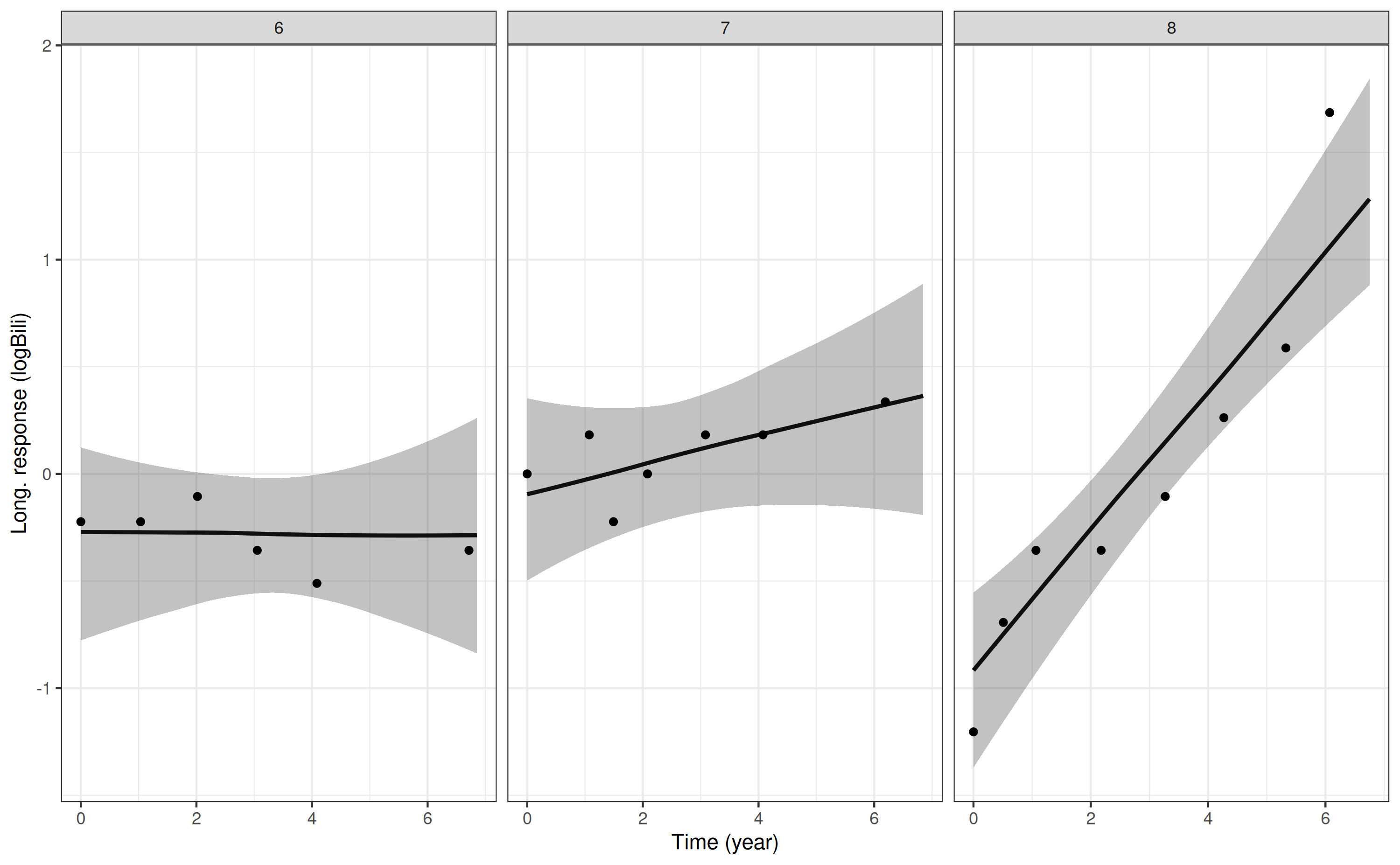
and here are the plots for serum albumin:
p2 <- posterior_traj(mod3, m = 2, ids = 6:8)
pp2 <- plot(p2, plot_observed = TRUE)
pp2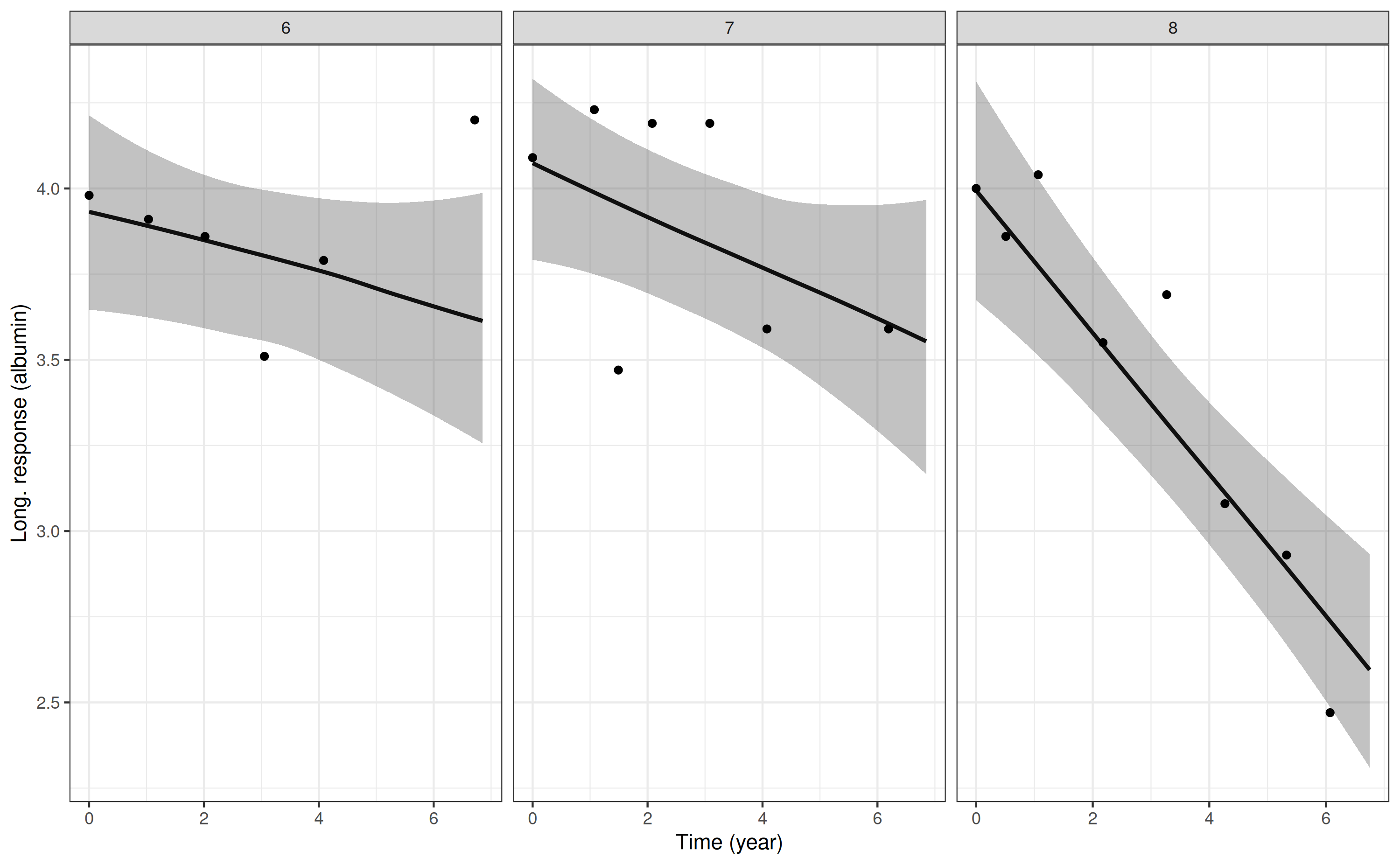
The m argument specifies which biomarker we want to
predict for (only relevant for a multivariate joint model). The
ids argument is optional, and specifies a subset of
individuals for whom we want to predict. In the plotting method, the
plot_observed = TRUE specifies that we want to include the
observed biomarker values in the plot of the longitudinal
trajectory.
If we wanted to extrapolate the trajectory forward from the event or
censoring time for each individual, then this can be easily achieved by
specifying extrapolate = TRUE in the
posterior_traj call. For example, here is the plot for log
serum bilirubin with extrapolation:
p3 <- posterior_traj(mod3, m = 1, ids = 6:8, extrapolate = TRUE)
pp3 <- plot(p3, plot_observed = TRUE, vline = TRUE)
pp3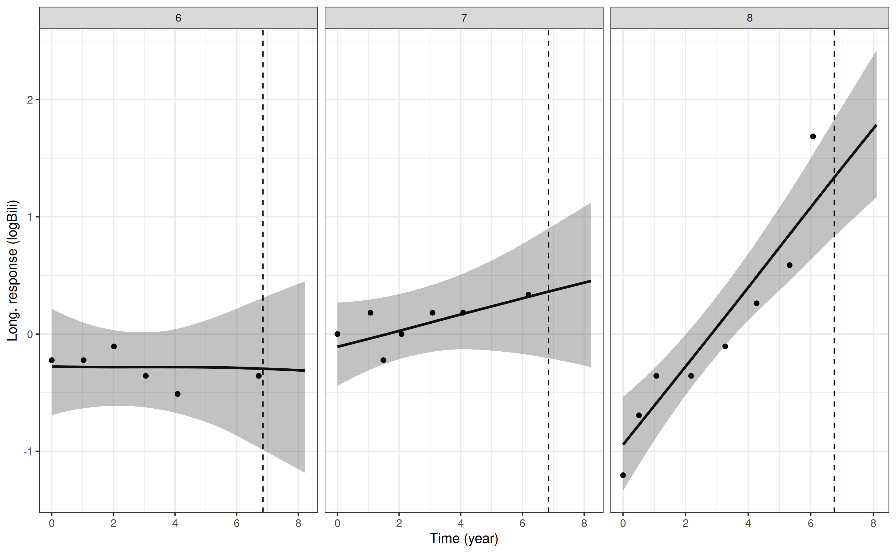
and for serum albumin with extrapolation:
p4 <- posterior_traj(mod3, m = 2, ids = 6:8, extrapolate = TRUE)
pp4 <- plot(p4, plot_observed = TRUE, vline = TRUE)
pp4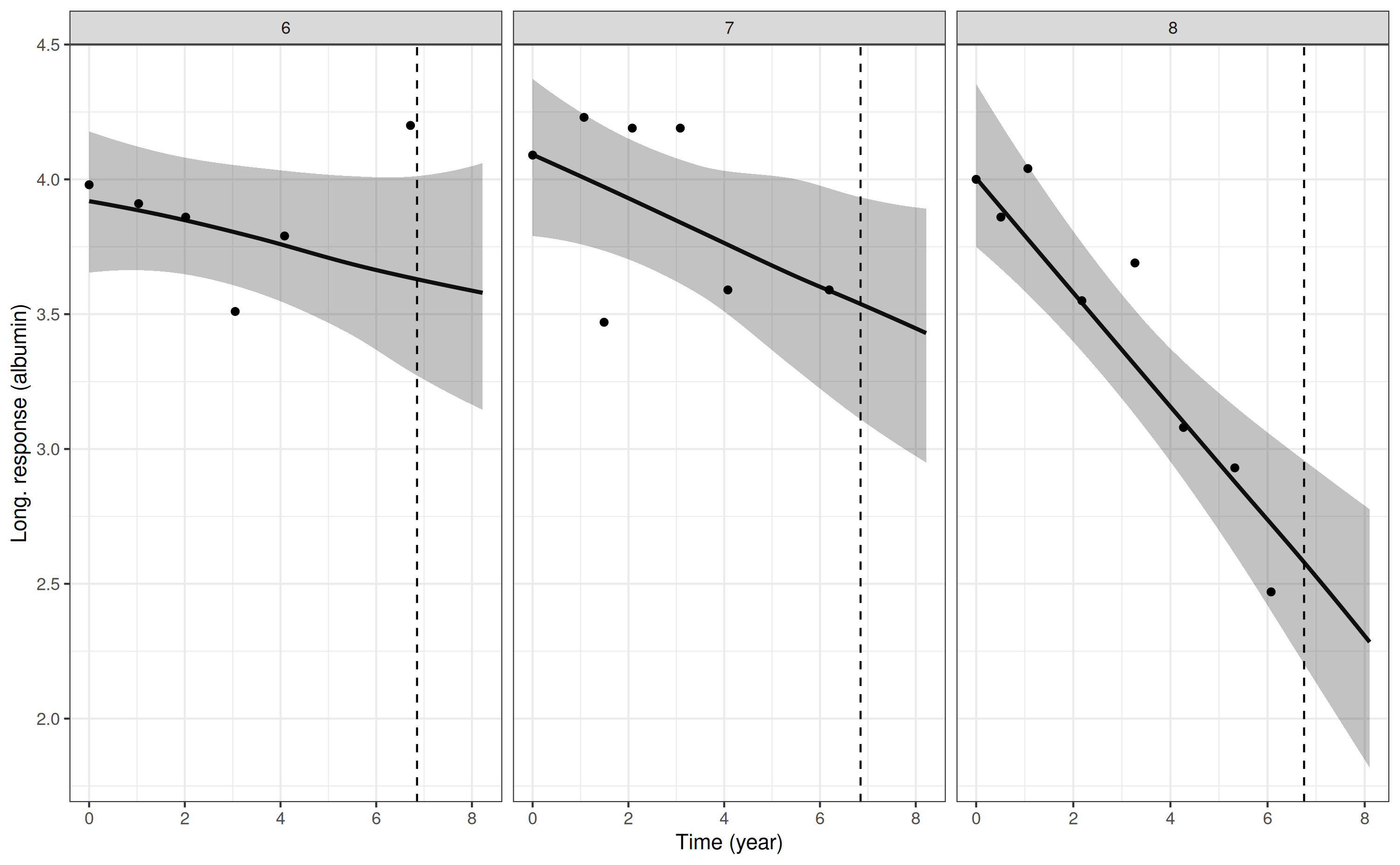
Here, we included the vline = TRUE which adds a vertical
dashed line at the timing of the individual’s event or censoring time.
The interpolation and extrapolation of the biomarker trajectory can be
further controlled through the control argument to the
posterior_traj function; for example, we could specify the
number of time points at which to predict, the distance by which to
extrapolate, and so on.
We could customize these plots further, for example, by using any of
the ggplot2 functionality or using the additional
arguments described in help(plot.predict.stanjm).
Predicted individual-specific survival curves for in-sample individuals
Predicted individual-specific survival probabilities and/or survival
curves can be obtained using the posterior_survfit
function. The function by default returns a data frame with the
individual ID, the time, and the predicted survival probability
(posterior mean and limits for the 95% credible interval). The
uncertainty level for the credible interval can be changed via the
prob argument. By default, individual-specific survival
probabilities are calculated conditional on the individual’s
last known survival time. When we are predicting survival probabilities
for individuals that were used in the estimation of the model
(i.e. in-sample individuals, where no new covariate data is provided),
then the individual’s “last known survival time” will be their event or
censoring time. (Note that if we wanted didn’t want to condition on the
individual’s last known survival time, then we could specify
condition = FALSE, but we probably wouldn’t want to do this
unless we were calculating marginal or standardised survival
probabilities, which are discussed later).
The default argument extrapolate = TRUE specifies that
the individual-specific conditional survival probabilities will be
calculated at evenly spaced time points between the individual’s last
known survival time and the maximum follow up time that was observed in
the estimation sample. The behaviour of the extrapolation can be further
controlled via the control argument. If we were to specify
extrapolate = FALSE then the survival probabilities would
only be calculated at one time point, which could be specified in the
times argument (or otherwise would default to the
individual’s last known survival time).
As an example, let plot the predicted individual-specific conditional
survival curve for the same three individual’s that were used in the
previous example. The predicted survival curve will be obtained under
the multivariate joint model estimated above.
p5 <- posterior_survfit(mod3, ids = 6:8)
pp5 <- plot(p5)
pp5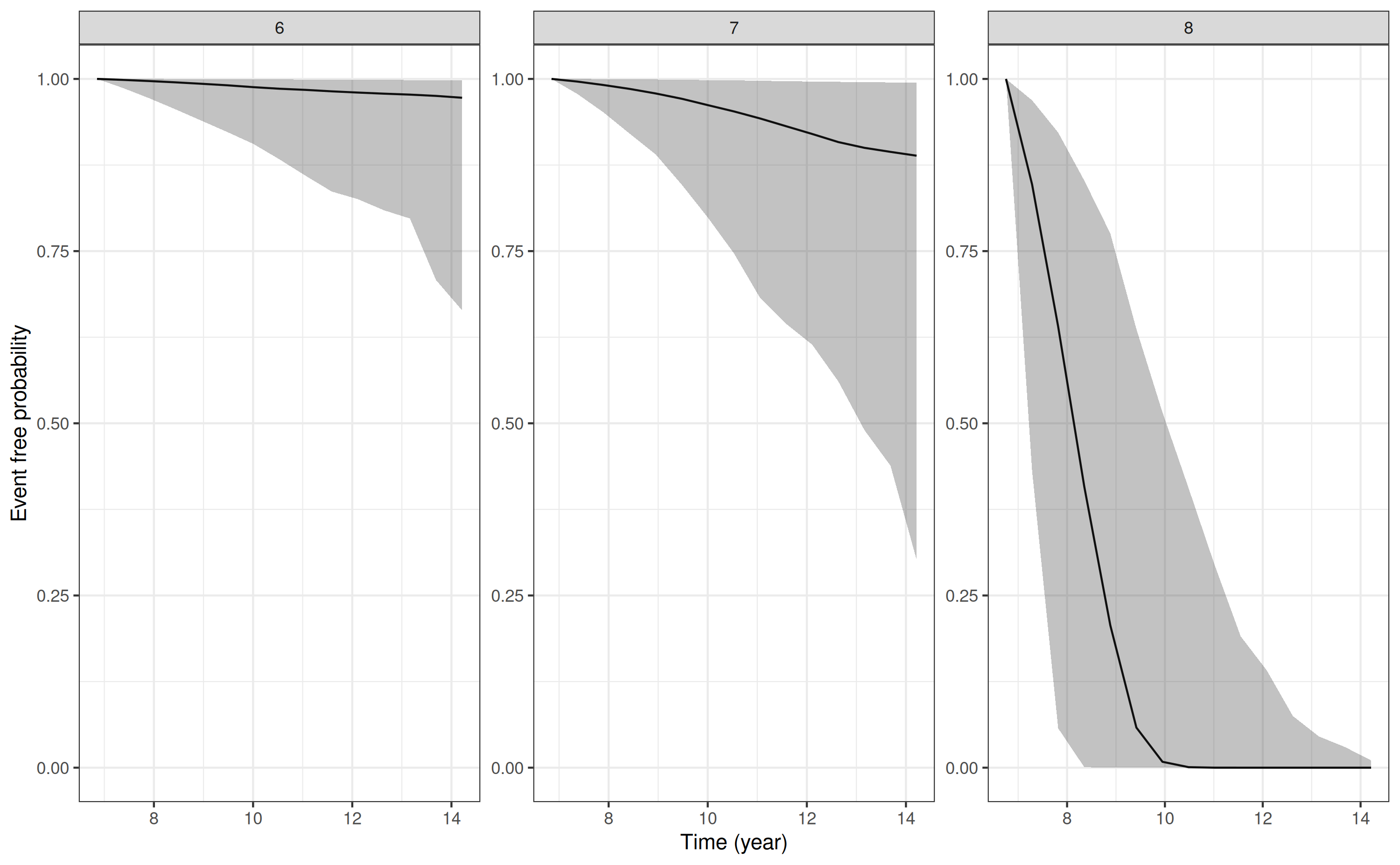
We could customize the plot further, for example, by using any of the
ggplot2 functionality or using the additional arguments
described in help(plot.survfit.stanjm).
Combined plot of longitudinal trajectories and survival curves
The package also provides a convenience plotting function, which combines plots of the individual-specific longitudinal trajectories, and the individual-specific survival function. We can demonstrate this by replotting the predictions for the three individuals in the previous example:
plot_stack_jm(yplot = list(pp3, pp4), survplot = pp5)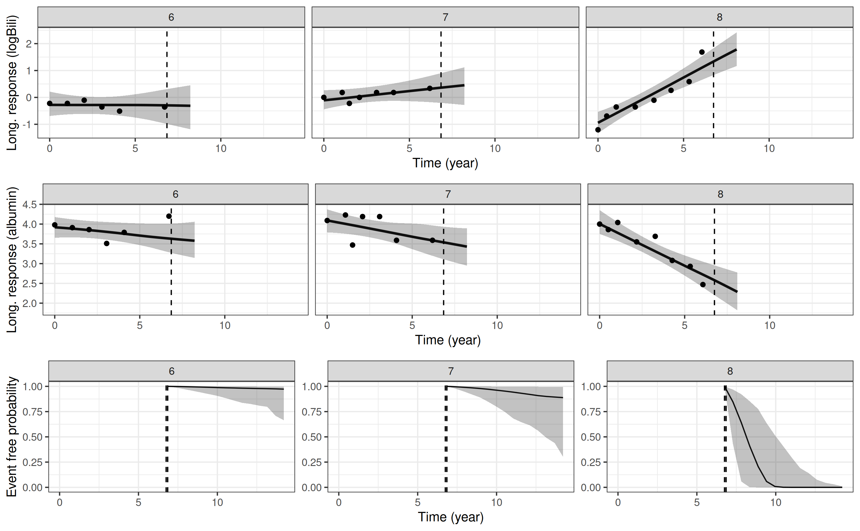
Here we can see the strong relationship between the underlying values
of the biomarkers and mortality. Patient 8 who, relative to
patients 6 and 7, has a higher underlying
value for log serum bilirubin and a lower underlying value for serum
albumin at the end of their follow up has a far worse predicted
probability of survival.
Predicted individual-specific longitudinal trajectory and survival curve for out-of-sample individuals (i.e. dynamic predictions)
Let us take an individual from our training data, in this case the
individual with subject ID value 8. However, we will
pretend this individual was not a member of our training data and rather
that they are a new individual for whom we have obtained new biomarker
measurements. Our goal is to obtain predictions for the longitudinal
trajectory for this individual, and their conditional survival curve,
given that we know they are conditional on their biomarker measurements
we currently have available.
First, let’s extract the data for subject 8 and then
rename their subject ID value so that they appear to be an individual
who was not included in our training dataset:
ndL <- pbcLong[pbcLong$id == 8, , drop = FALSE]
ndE <- pbcSurv[pbcSurv$id == 8, , drop = FALSE]
ndL$id <- paste0("new_patient")
ndE$id <- paste0("new_patient")
Note that we have both the longitudinal data and event data for this
new individual. We require data for both submodels because we are going
to generate dynamic predictions that require drawing new
individual-specific parameters (i.e. random effects) for this individual
conditional on their observed data. That means we need to evaluate the
likelihood for the full joint model and that requires both the
longitudinal and event data (note however that the status indicator
death will be ignored, since it is assumed that the
individual we are predicting for is still alive at the time we wish to
generate the predictions).
Now we can pass this data to the posterior_traj function
in the same way as for the in-sample individuals, except we will now
specify the newdataLong and newdataEvent
arguments. We will also specify the last_time argument so
that the function knows which variable in the event data specifies the
individual’s last known survival time (the default behaviour is to use
the time of the last biomarker measurement).
Our predictions for this new individual for the log serum bilirubin trajectory can be obtained using:
p6 <- posterior_traj(mod3, m = 1,
                     newdataLong = ndL,
                     newdataEvent = ndE,
                     last_time = "futimeYears")
Drawing new random effects for 1 individuals. Monitoring progress:
| | | 0% | |======================================================================| 100%
pp6 <- plot(p6, plot_observed = TRUE, vline = TRUE)
pp6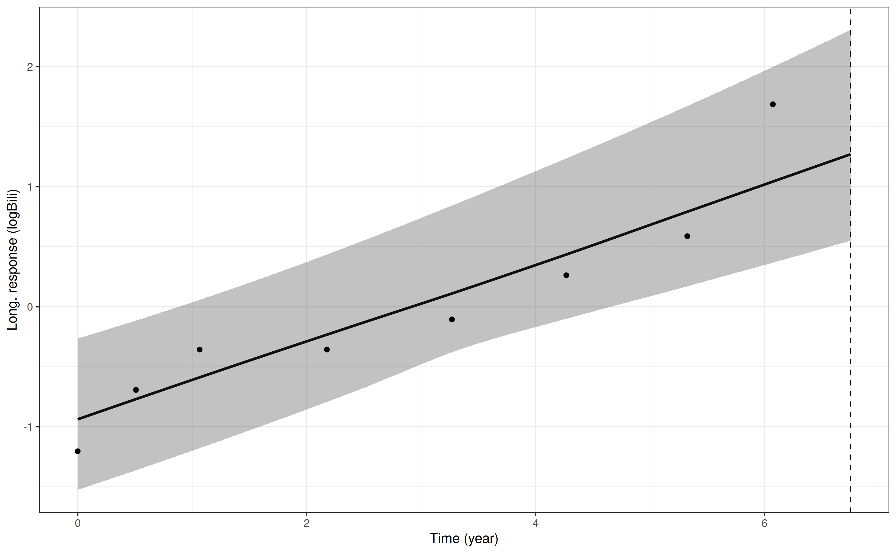
and for the serum albumin trajectory:
p7 <- posterior_traj(mod3, m = 2,
                     newdataLong = ndL,
                     newdataEvent = ndE,
                     last_time = "futimeYears")
Drawing new random effects for 1 individuals. Monitoring progress:
| | | 0% | |======================================================================| 100%
pp7 <- plot(p7, plot_observed = TRUE, vline = TRUE)
pp7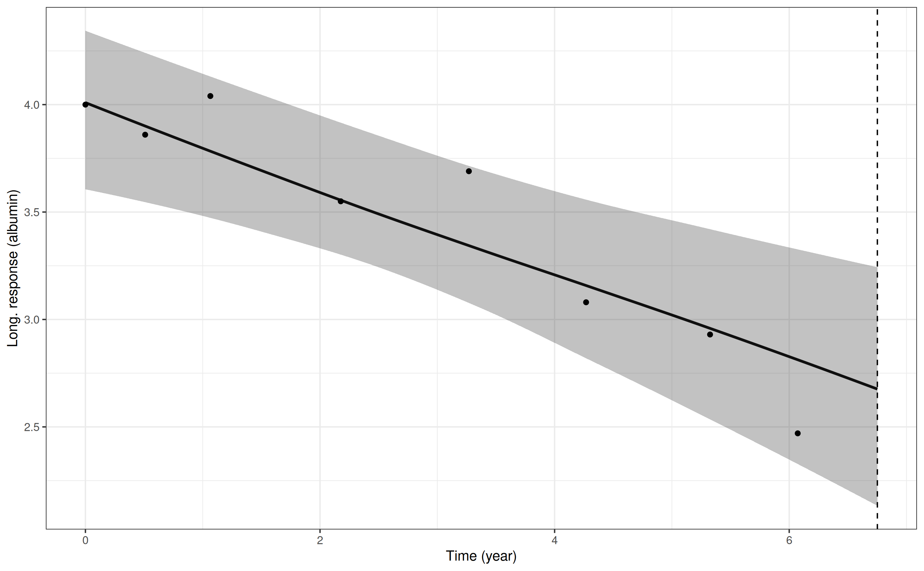
For the conditional survival probabilities we use similar
information, provided to the posterior_survfit
function:
p8 <- posterior_survfit(mod3,
                        newdataLong = ndL,
                        newdataEvent = ndE,
                        last_time = "futimeYears")
Drawing new random effects for 1 individuals. Monitoring progress:
| | | 0% | |======================================================================| 100%
pp8 <- plot(p8)
pp8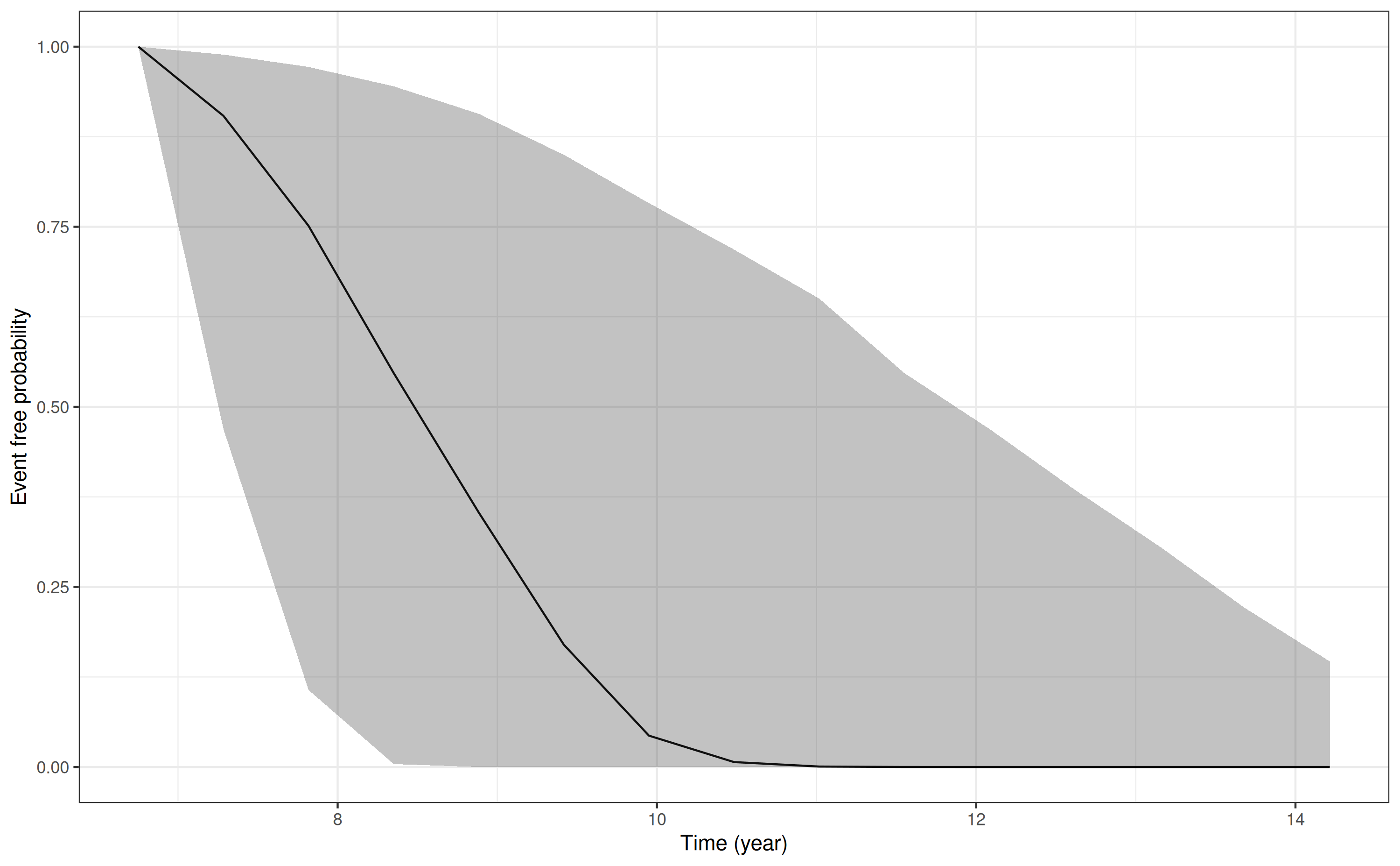
We can then use the plot_stack_jm function, as we saw in
a previous example, to stack the plots of the longitudinal trajectory
and the conditional survival curve:
plot_stack_jm(yplot = list(pp6, pp7), survplot = pp8)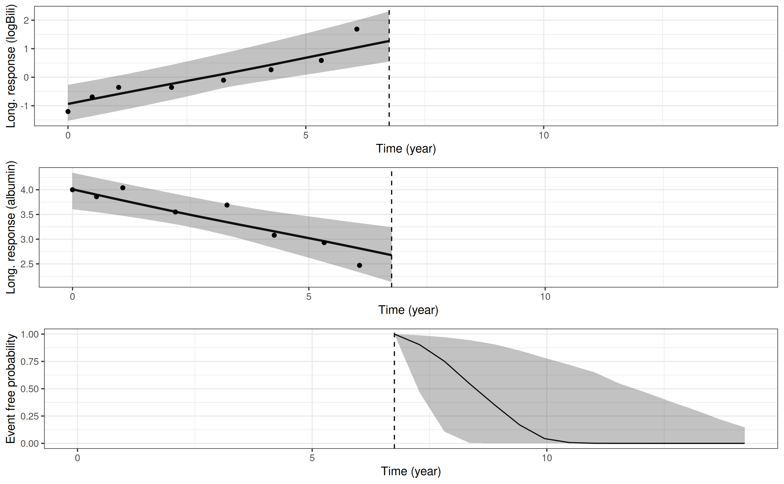
Here we see that the predicted longitudinal trajectories and conditional survival curve for this individual, obtained using the dynamic predictions approach, are similar to the predictions we obtained when we used their individual-specific parameters from the original model estimation. This is because in both situations we are conditioning on the same outcome data.
Side note: We can even compare the estimated
individual specific parameters obtained under the two approaches. For
example, here is the posterior mean for the estimated
individual-specific parameters for individual 8 from the
fitted model:
$`(Intercept)`
[1] -1.636025

$year
[1] 0.1106856

$`(Intercept)`
[1] 0.4636367

$year
[1] -0.04915748
and here is the mean of the draws for the individual-specific
parameters for individual 8 under the dynamic predictions
approach:
b[Long1|(Intercept) id:new_patient]        b[Long1|year id:new_patient]
                        -1.65217893                          0.10504485
b[Long2|(Intercept) id:new_patient]        b[Long2|year id:new_patient]
                         0.45330164                         -0.03059108
Predicted population-level longitudinal trajectory
Suppose we wanted to predict the longitudinal trajectory for each of
the biomarkers, marginalising over the distribution of the
individual-specific parameters. To do this, we can pass a new data frame
with the covariate values we want to use in the predictions. Here, we
will demonstrate this by obtaining the predicted trajectory for log
serum bilirubin, under the multivariate joint model that was estimated
previously. Our prediction data will require the variables
year, sex and trt, since these
were the covariates used in the longitudinal submodel.
We will predict the value of log serum bilirubin at years 0 through
10, for each combination of sex and trt. We
also need to include the id variable in our prediction data
because this is relevant to the longitudinal submodel. Since we want to
marginalise over the individual-specific parameters
(i.e. individual-level random effects) we need to note two things:
First, the values for the
idvariable must not match any individual used in the model estimation. Here, we use the followingidvalues:"male_notrt","female_notrt","male_trt", and"female_trt", since each individual in our prediction data represents a different combination ofsexandtrt. However, we could have given the individuals anyidvalue just as long as is didn’t match an individual who was used in the model estimationSecond, we need to specify the argument
dynamic = FALSEwhen callingposterior_traj. This specifies that we do not want to draw new individual-specific parameters conditional on outcome data observed up to some time \(t\). Instead, we want predictions that marginalise over the distribution of individual-specific parameters and are therefore conditional only on covariates and not conditional on outcome data for the new individuals.
Here is our prediction data:
ndL <- expand.grid(year = seq(0, 10, 1),
                   sex = c("m", "f"),
                   trt = 0:1)
ndL$id <- rep(c("male_notrt", "female_notrt",
                "male_trt", "female_trt"), each = 11)
ndL <- ndL[, c(4,1,2,3)]
str(ndL)
'data.frame': 44 obs. of 4 variables:
$ id : chr "male_notrt" "male_notrt" "male_notrt" "male_notrt" ...
$ year: num 0 1 2 3 4 5 6 7 8 9 ...
$ sex : Factor w/ 2 levels "m","f": 1 1 1 1 1 1 1 1 1 1 ...
$ trt : int 0 0 0 0 0 0 0 0 0 0 ...And to predict the marginal longitudinal trajectory for log serum bilirubin under each covariate profile and plot it we can type:
p1 <- posterior_traj(mod3, m = 1, newdataLong = ndL, dynamic = FALSE)
plot(p1) + ggplot2::coord_cartesian(ylim = c(-10,15))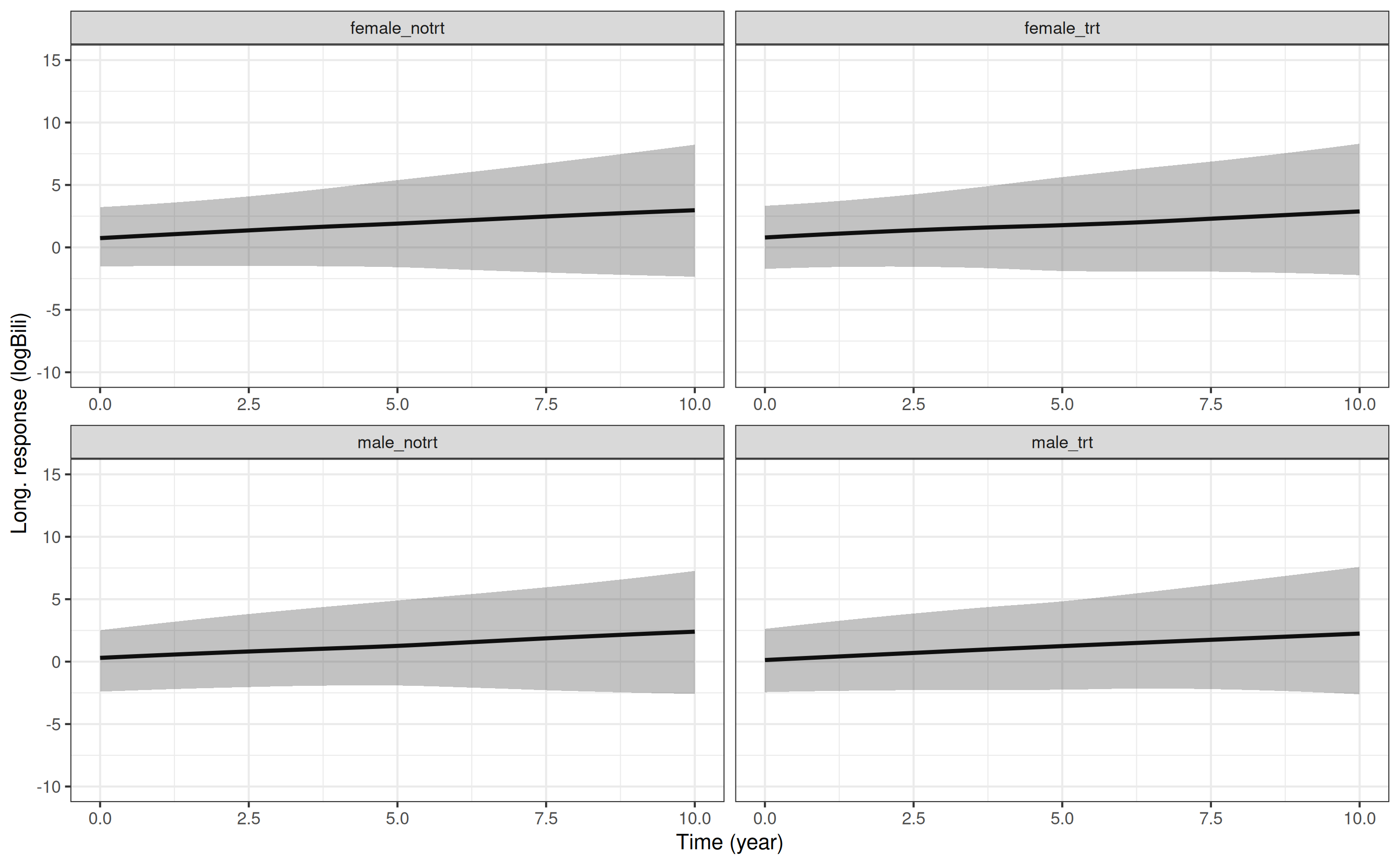
Because we are marginalising over the distribution of the
individual-specific parameters, we are incorporating all the variation
related to between-individual differences, and therefore the prediction
interval is wide (shown by the shaded area around the marginal
longitudinal trajectory). The magnitude of the effects of both
sex and trt are relatively small compared to
the population-level effect of year and the
between-individual variation in the intercept and slope. For example,
here are the point estimates for the population-level effects of
sex, trt, and year:
fixef(mod3)$Long1(Intercept) sexf trt year
0.26316891 0.47545756 -0.06287211 0.22199841 and here are the standard deviations for the individual-level random effects:
VarCorr(mod3) Groups Name Std.Dev. Corr
id Long1|(Intercept) 1.241233
Long1|year 0.188221 0.490
Long2|(Intercept) 0.513955 -0.652 -0.494
Long2|year 0.096057 -0.567 -0.810 0.454This shows us that the point estimates for the population-level
effects of sex and trt are 0.57 and -0.10,
respectively, whereas the standard deviation for the individual-specific
intercept and slope parameters are 1.24 and 0.19; hence, any differences
due to the population-level effects of gender and treatment
(i.e. differences in the black line across the four panels of the plot)
are swamped by the width of the uncertainty intervals (i.e. the grey
shaded areas).
Standardised survival curves
In this example we show how a standardised survival curve can be
obtained, where the \(i =
1,...,N^{pred}\) individuals used in generating the standardised
survival curve are the same individuals that were used in estimating the
model. We will obtain the survival curve for the multivariate joint
model estimated in an earlier example (mod3). The
standardise = TRUE argument to
posterior_survfit specifies that we want to obtain
individual-specific predictions of the survival curve and then average
these. Because, in practical terms, we need to obtain survival
probabilities at time \(t\) for each
individual and then average them we want to explicitly specify the
values of \(t\) we want to use (and the
same values of \(t\) will be used for
individuals). We specify the values of \(t\) to use via the times
argument; here we will predict the standardised survival curve at time 0
and then for convenience we can just specify
extrapolate = TRUE (which is the default anyway) which will
mean we automatically predict at 10 evenly spaced time points between 0
and the maximum event or censoring time.
p1 <- posterior_survfit(mod3, standardise = TRUE, times = 0)
head(p1) # data frame with standardised survival probabilities
year survpred ci_lb ci_ub
1 0.0000 1.0000 1.0000 1.0000
2 1.0154 0.8243 0.7659 0.8943
3 2.0307 0.7309 0.6606 0.7805
4 3.0461 0.6789 0.6133 0.7221
5 4.0614 0.6351 0.5746 0.6877
6 5.0768 0.5934 0.5386 0.6456
plot(p1) # plot the standardised survival curve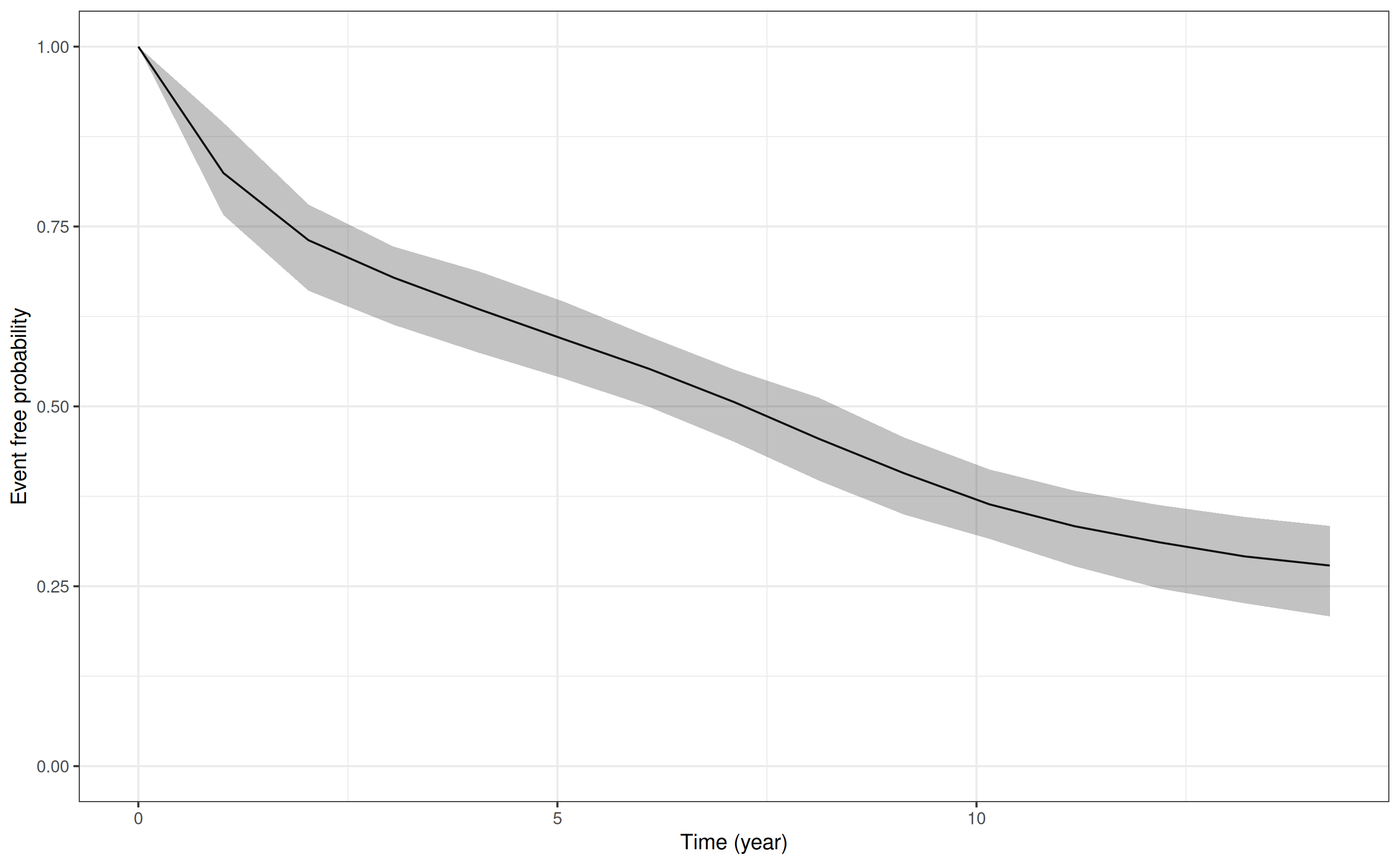
References
- Henderson R, Diggle P, Dobson A. Joint modelling of longitudinal measurements and event time data. Biostatistics 2000;1(4):465-80.
- Wulfsohn MS, Tsiatis AA. A joint model for survival and longitudinal data measured with error. Biometrics 1997;53(1):330-9.
- Tsiatis AA, Davidian M. Joint modeling of longitudinal and time-to-event data: An overview. Stat Sinica 2004;14(3):809-34.
- Gould AL, Boye ME, Crowther MJ, Ibrahim JG, Quartey G, Micallef S, et al. Joint modeling of survival and longitudinal non-survival data: current methods and issues. Report of the DIA Bayesian joint modeling working group. Stat Med. 2015;34(14):2181-95.
- Rizopoulos D. Joint Models for Longitudinal and Time-to-Event Data: With Applications in R CRC Press; 2012.
- Liu G, Gould AL. Comparison of alternative strategies for analysis of longitudinal trials with dropouts. J Biopharm Stat 2002;12(2):207-26.
- Prentice RL. Covariate Measurement Errors and Parameter-Estimation in a Failure Time Regression-Model. Biometrika 1982;69(2):331-42.
- Baraldi AN, Enders CK. An introduction to modern missing data analyses. J Sch Psychol 2010;48(1):5-37.
- Philipson PM, Ho WK, Henderson R. Comparative review of methods for handling drop-out in longitudinal studies. Stat Med 2008;27(30):6276-98.
- Pantazis N, Touloumi G. Bivariate modelling of longitudinal measurements of two human immunodeficiency type 1 disease progression markers in the presence of informative drop-outs. Applied Statistics 2005;54:405-23.
- Taylor JM, Park Y, Ankerst DP, et al. Real-time individual predictions of prostate cancer recurrence using joint models. Biometrics 2013;69(1):206-13.
- Brilleman SL, Crowther MJ, Moreno-Betancur M, Buros Novik J, Wolfe R. Joint longitudinal and time-to-event models via Stan. In: Proceedings of StanCon 2018. https://github.com/stan-dev/stancon_talks
- Stan Development Team. rstanarm: Bayesian applied regression modeling via Stan. R package version 2.14.1. https://mc-stan.org/. 2016.
- R Core Team. R: A language and environment for statistical computing. Vienna, Austria: R Foundation for Statistical Computing; 2015.
- Crowther MJ, Lambert PC, Abrams KR. Adjusting for measurement error in baseline prognostic biomarkers included in a time-to-event analysis: a joint modelling approach. BMC Med Res Methodol 2013;13.
- Hickey GL, Philipson P, Jorgensen A, Kolamunnage-Dona R. Joint modelling of time-to-event and multivariate longitudinal outcomes: recent developments and issues. BMC Med Res Methodol 2016;16(1):117.
- Rizopoulos D, Ghosh P. A Bayesian semiparametric multivariate joint model for multiple longitudinal outcomes and a time-to-event. Stat Med. 2011;30(12):1366-80.
- Laurie DP. Calculation of Gauss-Kronrod quadrature rules. Math Comput 1997;66(219):1133-45.
- Rizopoulos D. Dynamic Predictions and Prospective Accuracy in Joint Models for Longitudinal and Time-to-Event Data. Biometrics 2011;67(3):819-829.
- Therneau T, Grambsch P. Modeling Survival Data: Extending the Cox Model Springer-Verlag, New York; 2000. ISBN: 0-387-98784-3