In-sample or out-of-sample predictive errors

This is a convenience function for computing \(y - y^{rep}\) (in-sample, for observed \(y\)) or \(y - \tilde{y}\) (out-of-sample, for new or held-out \(y\)). The method for stanreg objects calls posterior_predict internally, whereas the method for matrices accepts the matrix returned by posterior_predict as input and can be used to avoid multiple calls to posterior_predict.

Usage

# S3 method for class 'stanreg'
predictive_error(
  object,
  newdata = NULL,
  draws = NULL,
  re.form = NULL,
  seed = NULL,
  offset = NULL,
  ...
)

# S3 method for class 'matrix'
predictive_error(object, y, ...)

# S3 method for class 'ppd'
predictive_error(object, y, ...)

Arguments

object: Either a fitted model object returned by one of the rstanarm modeling functions (a stanreg object) or, for the matrix method, a matrix of draws from the posterior predictive distribution returned by posterior_predict.
newdata, draws, seed, offset, re.form: Optional arguments passed to posterior_predict. For binomial models, please see the Note section below if newdata will be specified.
...: Currently ignored.
y: For the matrix method only, a vector of \(y\) values the same length as the number of columns in the matrix used as object. The method for stanreg objects takes y directly from the fitted model object.

Value

A draws by nrow(newdata) matrix. If newdata is not specified then it will be draws by nobs(object).

Note

The Note section in posterior_predict about newdata for binomial models also applies for predictive_error, with one important difference. For posterior_predict if the left-hand side of the model formula is cbind(successes, failures) then the particular values of successes and failures in newdata don't matter, only that they add to the desired number of trials. This is not the case for predictive_error. For predictive_error the particular value of successes matters because it is used as \(y\) when computing the error.

Examples

if (.Platform$OS.type != "windows" || .Platform$r_arch != "i386") {
if (!exists("example_model")) example(example_model)
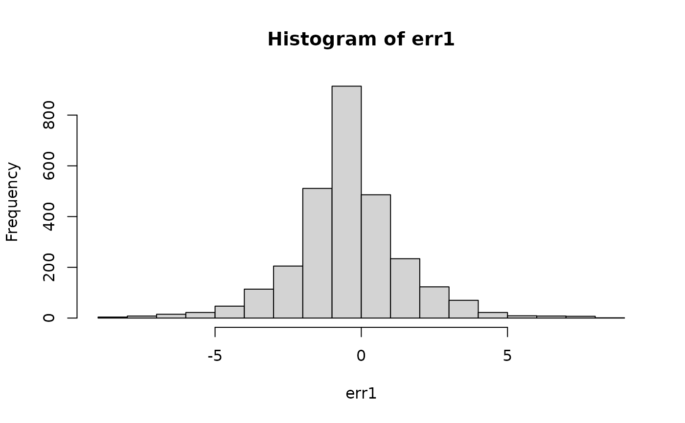
err1 <- predictive_error(example_model, draws = 50)
hist(err1)

# Using newdata with a binomial model
formula(example_model)
nd <- data.frame(
 size = c(10, 20), 
 incidence = c(5, 10), 
 period = factor(c(1,2)), 
 herd = c(1, 15)
)
err2 <- predictive_error(example_model, newdata = nd, draws = 10, seed = 1234)

# stanreg vs matrix methods
fit <- stan_glm(mpg ~ wt, data = mtcars, iter = 300)
preds <- posterior_predict(fit, seed = 123)
all.equal(
  predictive_error(fit, seed = 123),
  predictive_error(preds, y = fit$y)
)
}

#> 
#> SAMPLING FOR MODEL 'continuous' NOW (CHAIN 1).
#> Chain 1: 
#> Chain 1: Gradient evaluation took 2e-05 seconds
#> Chain 1: 1000 transitions using 10 leapfrog steps per transition would take 0.2 seconds.
#> Chain 1: Adjust your expectations accordingly!
#> Chain 1: 
#> Chain 1: 
#> Chain 1: Iteration:   1 / 300 [  0%]  (Warmup)
#> Chain 1: Iteration:  30 / 300 [ 10%]  (Warmup)
#> Chain 1: Iteration:  60 / 300 [ 20%]  (Warmup)
#> Chain 1: Iteration:  90 / 300 [ 30%]  (Warmup)
#> Chain 1: Iteration: 120 / 300 [ 40%]  (Warmup)
#> Chain 1: Iteration: 150 / 300 [ 50%]  (Warmup)
#> Chain 1: Iteration: 151 / 300 [ 50%]  (Sampling)
#> Chain 1: Iteration: 180 / 300 [ 60%]  (Sampling)
#> Chain 1: Iteration: 210 / 300 [ 70%]  (Sampling)
#> Chain 1: Iteration: 240 / 300 [ 80%]  (Sampling)
#> Chain 1: Iteration: 270 / 300 [ 90%]  (Sampling)
#> Chain 1: Iteration: 300 / 300 [100%]  (Sampling)
#> Chain 1: 
#> Chain 1:  Elapsed Time: 0.008 seconds (Warm-up)
#> Chain 1:                0.004 seconds (Sampling)
#> Chain 1:                0.012 seconds (Total)
#> Chain 1: 
#> 
#> SAMPLING FOR MODEL 'continuous' NOW (CHAIN 2).
#> Chain 2: 
#> Chain 2: Gradient evaluation took 8e-06 seconds
#> Chain 2: 1000 transitions using 10 leapfrog steps per transition would take 0.08 seconds.
#> Chain 2: Adjust your expectations accordingly!
#> Chain 2: 
#> Chain 2: 
#> Chain 2: Iteration:   1 / 300 [  0%]  (Warmup)
#> Chain 2: Iteration:  30 / 300 [ 10%]  (Warmup)
#> Chain 2: Iteration:  60 / 300 [ 20%]  (Warmup)
#> Chain 2: Iteration:  90 / 300 [ 30%]  (Warmup)
#> Chain 2: Iteration: 120 / 300 [ 40%]  (Warmup)
#> Chain 2: Iteration: 150 / 300 [ 50%]  (Warmup)
#> Chain 2: Iteration: 151 / 300 [ 50%]  (Sampling)
#> Chain 2: Iteration: 180 / 300 [ 60%]  (Sampling)
#> Chain 2: Iteration: 210 / 300 [ 70%]  (Sampling)
#> Chain 2: Iteration: 240 / 300 [ 80%]  (Sampling)
#> Chain 2: Iteration: 270 / 300 [ 90%]  (Sampling)
#> Chain 2: Iteration: 300 / 300 [100%]  (Sampling)
#> Chain 2: 
#> Chain 2:  Elapsed Time: 0.008 seconds (Warm-up)
#> Chain 2:                0.004 seconds (Sampling)
#> Chain 2:                0.012 seconds (Total)
#> Chain 2: 
#> 
#> SAMPLING FOR MODEL 'continuous' NOW (CHAIN 3).
#> Chain 3: 
#> Chain 3: Gradient evaluation took 8e-06 seconds
#> Chain 3: 1000 transitions using 10 leapfrog steps per transition would take 0.08 seconds.
#> Chain 3: Adjust your expectations accordingly!
#> Chain 3: 
#> Chain 3: 
#> Chain 3: Iteration:   1 / 300 [  0%]  (Warmup)
#> Chain 3: Iteration:  30 / 300 [ 10%]  (Warmup)
#> Chain 3: Iteration:  60 / 300 [ 20%]  (Warmup)
#> Chain 3: Iteration:  90 / 300 [ 30%]  (Warmup)
#> Chain 3: Iteration: 120 / 300 [ 40%]  (Warmup)
#> Chain 3: Iteration: 150 / 300 [ 50%]  (Warmup)
#> Chain 3: Iteration: 151 / 300 [ 50%]  (Sampling)
#> Chain 3: Iteration: 180 / 300 [ 60%]  (Sampling)
#> Chain 3: Iteration: 210 / 300 [ 70%]  (Sampling)
#> Chain 3: Iteration: 240 / 300 [ 80%]  (Sampling)
#> Chain 3: Iteration: 270 / 300 [ 90%]  (Sampling)
#> Chain 3: Iteration: 300 / 300 [100%]  (Sampling)
#> Chain 3: 
#> Chain 3:  Elapsed Time: 0.009 seconds (Warm-up)
#> Chain 3:                0.004 seconds (Sampling)
#> Chain 3:                0.013 seconds (Total)
#> Chain 3: 
#> 
#> SAMPLING FOR MODEL 'continuous' NOW (CHAIN 4).
#> Chain 4: 
#> Chain 4: Gradient evaluation took 8e-06 seconds
#> Chain 4: 1000 transitions using 10 leapfrog steps per transition would take 0.08 seconds.
#> Chain 4: Adjust your expectations accordingly!
#> Chain 4: 
#> Chain 4: 
#> Chain 4: Iteration:   1 / 300 [  0%]  (Warmup)
#> Chain 4: Iteration:  30 / 300 [ 10%]  (Warmup)
#> Chain 4: Iteration:  60 / 300 [ 20%]  (Warmup)
#> Chain 4: Iteration:  90 / 300 [ 30%]  (Warmup)
#> Chain 4: Iteration: 120 / 300 [ 40%]  (Warmup)
#> Chain 4: Iteration: 150 / 300 [ 50%]  (Warmup)
#> Chain 4: Iteration: 151 / 300 [ 50%]  (Sampling)
#> Chain 4: Iteration: 180 / 300 [ 60%]  (Sampling)
#> Chain 4: Iteration: 210 / 300 [ 70%]  (Sampling)
#> Chain 4: Iteration: 240 / 300 [ 80%]  (Sampling)
#> Chain 4: Iteration: 270 / 300 [ 90%]  (Sampling)
#> Chain 4: Iteration: 300 / 300 [100%]  (Sampling)
#> Chain 4: 
#> Chain 4:  Elapsed Time: 0.006 seconds (Warm-up)
#> Chain 4:                0.004 seconds (Sampling)
#> Chain 4:                0.01 seconds (Total)
#> Chain 4: 
#> Warning: Bulk Effective Samples Size (ESS) is too low, indicating posterior means and medians may be unreliable.
#> Running the chains for more iterations may help. See
#> https://mc-stan.org/misc/warnings.html#bulk-ess
#> Warning: Tail Effective Samples Size (ESS) is too low, indicating posterior variances and tail quantiles may be unreliable.
#> Running the chains for more iterations may help. See
#> https://mc-stan.org/misc/warnings.html#tail-ess
#> [1] TRUE

Usage

Arguments

Value

Note

See also

Examples