Estimate subject-specific or standardised survival probabilities

This function allows us to generate estimated survival probabilities based on draws from the posterior predictive distribution. By default the survival probabilities are conditional on an individual's group-specific coefficients (i.e. their individual-level random effects). If prediction data is provided via the newdataLong and newdataEvent arguments, then the default behaviour is to sample new group-specific coefficients for the individuals in the new data using a Monte Carlo scheme that conditions on their longitudinal outcome data provided in newdataLong (sometimes referred to as "dynamic predictions", see Rizopoulos (2011)). This default behaviour can be stopped by specifying dynamic = FALSE, in which case the predicted survival probabilities will be marginalised over the distribution of the group-specific coefficients. This has the benefit that the user does not need to provide longitudinal outcome measurements for the new individuals, however, it does mean that the predictions will incorporate all the uncertainty associated with between-individual variation, since the predictions aren't conditional on any observed data for the individual. In addition, by default, the predicted subject-specific survival probabilities are conditional on observed values of the fixed effect covariates (ie, the predictions will be obtained using either the design matrices used in the original stan_jm model call, or using the covariate values provided in the newdataLong and newdataEvent arguments). However, if you wish to average over the observed distribution of the fixed effect covariates then this is possible – such predictions are sometimes referred to as standardised survival probabilties – see the standardise argument below.

Usage

posterior_survfit(
  object,
  newdataLong = NULL,
  newdataEvent = NULL,
  extrapolate = TRUE,
  control = list(),
  condition = NULL,
  last_time = NULL,
  prob = 0.95,
  ids,
  times = NULL,
  standardise = FALSE,
  dynamic = TRUE,
  scale = 1.5,
  draws = NULL,
  seed = NULL,
  ...
)

Arguments

object

A fitted model object returned by the stan_jm modelling function. See stanreg-objects.

newdataLong, newdataEvent

Optionally, a data frame (or in the case of newdataLong this can be a list of data frames) in which to look for variables with which to predict. If omitted, the model matrices are used. If new data is provided, then it should also contain the longitudinal outcome data on which to condition when drawing the new group-specific coefficients for individuals in the new data. Note that there is only allowed to be one row of data for each individual in newdataEvent, that is, time-varying covariates are not allowed in the prediction data for the event submodel. Also, newdataEvent can optionally include a variable with information about the last known survival time for the new individuals – see the description for the last_time argument below – however also note that when generating the survival probabilities it is of course assumed that all individuals in newdataEvent have not yet experienced the event (that is, any variable in newdataEvent that corresponds to the event indicator will be ignored).

extrapolate

A logical specifying whether to extrapolate the estimated survival probabilities beyond the times specified in the times argument. If TRUE then the extrapolation can be further controlled using the control argument.

control

A named list with parameters controlling extrapolation of the estimated survival function when extrapolate = TRUE. The list can contain one or more of the following named elements:

epoints: a positive integer specifying the number of discrete time points at which to calculate the forecasted survival probabilities. The default is 10.
edist: a positive scalar specifying the amount of time across which to forecast the estimated survival function, represented in units of the time variable time_var (from fitting the model). The default is to extrapolate between the times specified in the times argument and the maximum event or censoring time in the original data. If edist leads to times that are beyond the maximum event or censoring time in the original data then the estimated survival probabilities will be truncated at that point, since the estimate for the baseline hazard is not available beyond that time.

condition

A logical specifying whether the estimated subject-specific survival probabilities at time t should be conditioned on survival up to a fixed time point u. The default is for condition to be set to TRUE, unless standardised survival probabilities have been requested (by specifying standardise = TRUE), in which case condition must (and will) be set to FALSE. When conditional survival probabilities are requested, the fixed time point u will be either: (i) the value specified via the last_time argument; or if the last_time argument is NULL then the latest observation time for each individual (taken to be the value in the times argument if newdataEvent is specified, or the observed event or censoring time if newdataEvent is NULL.

last_time

A scalar, character string, or NULL. This argument specifies the last known survival time for each individual when conditional predictions are being obtained. If newdataEvent is provided and conditional survival predictions are being obtained, then the last_time argument can be one of the following: (i) a scalar, this will use the same last time for each individual in newdataEvent; (ii) a character string, naming a column in newdataEvent in which to look for the last time for each individual; (iii) NULL, in which case the default is to use the time of the latest longitudinal observation in newdataLong. If newdataEvent is NULL then the last_time argument cannot be specified directly; instead it will be set equal to the event or censoring time for each individual in the dataset that was used to estimate the model. If standardised survival probabilities are requested (i.e. standardise = TRUE) then conditional survival probabilities are not allowed and therefore the last_time argument is ignored.

prob

A scalar between 0 and 1 specifying the width to use for the uncertainty interval (sometimes called credible interval) for the predictions. For example prob = 0.95 (the default) means that the 2.5th and 97.5th percentiles will be provided.

ids

An optional vector specifying a subset of IDs for whom the predictions should be obtained. The default is to predict for all individuals who were used in estimating the model or, if newdataLong and newdataEvent are specified, then all individuals contained in the new data.

times

A scalar, a character string, or NULL. Specifies the times at which the estimated survival probabilities should be calculated. It can be either: (i) NULL, in which case it will default to the last known survival time for each individual, as determined by the last_time argument; (ii) a scalar, specifying a time to estimate the survival probability for each of the individuals; or (iii) if newdataEvent is provided, it can be the name of a variable in newdataEvent that indicates the time at which the survival probabilities should be calculated for each individual.

standardise

A logical specifying whether the estimated subject-specific survival probabilities should be averaged across all individuals for whom the subject-specific predictions are being obtained. This can be used to average over the covariate and random effects distributions of the individuals used in estimating the model, or the individuals included in the newdata arguments. This approach of averaging across the observed distribution of the covariates is sometimes referred to as a "standardised" survival curve. If standardise = TRUE, then the times argument must be specified and it must be constant across individuals, that is, the survival probabilities must be calculated at the same time for all individuals.

dynamic

A logical that is only relevant if new data is provided via the newdataLong and newdataEvent arguments. If dynamic = TRUE, then new group-specific parameters are drawn for the individuals in the new data, conditional on their longitudinal biomarker data contained in newdataLong. These group-specific parameters are then used to generate individual-specific survival probabilities for these individuals. These are often referred to as "dynamic predictions" in the joint modelling context, because the predictions can be updated each time additional longitudinal biomarker data is collected on the individual. On the other hand, if dynamic = FALSE then the survival probabilities will just be marginalised over the distribution of the group-specific coefficients; this will mean that the predictions will incorporate all uncertainty due to between-individual variation so there will likely be very wide credible intervals on the predicted survival probabilities.

scale

A scalar, specifying how much to multiply the asymptotic variance-covariance matrix for the random effects by, which is then used as the "width" (ie. variance-covariance matrix) of the multivariate Student-t proposal distribution in the Metropolis-Hastings algorithm. This is only relevant when newdataEvent is supplied and dynamic = TRUE, in which case new random effects are simulated for the individuals in the new data using the Metropolis-Hastings algorithm.

draws

An integer indicating the number of MCMC draws to return. The default is to set the number of draws equal to 200, or equal to the size of the posterior sample if that is less than 200.

seed

An optional seed to use.

...

Currently unused.

Value

A data frame of class survfit.stanjm. The data frame includes columns for each of the following: (i) the median of the posterior predictions of the estimated survival probabilities (survpred); (ii) each of the lower and upper limits of the corresponding uncertainty interval for the estimated survival probabilities (ci_lb and ci_ub); (iii) a subject identifier (id_var), unless standardised survival probabilities were estimated; (iv) the time that the estimated survival probability is calculated for (time_var). The returned object also includes a number of additional attributes.

Note

Note that if any variables were transformed (e.g. rescaled) in the data used to fit the model, then these variables must also be transformed in newdataLong and newdataEvent. This only applies if variables were transformed before passing the data to one of the modeling functions and not if transformations were specified inside the model formula.

References

Rizopoulos, D. (2011). Dynamic predictions and prospective accuracy in joint models for longitudinal and time-to-event data. Biometrics 67, 819.

Examples

if (.Platform$OS.type != "windows" || .Platform$r_arch != "i386") {
# \donttest{
  # Run example model if not already loaded
  if (!exists("example_jm")) example(example_jm)

  # Obtain subject-specific survival probabilities for a few
  # selected individuals in the estimation dataset who were
  # known to survive up until their censoring time. By default
  # the posterior_survfit function will estimate the conditional
  # survival probabilities, that is, conditional on having survived
  # until the event or censoring time, and then by default will
  # extrapolate the survival predictions forward from there.
  ps1 <- posterior_survfit(example_jm, ids = c(7,13,15))
  # We can plot the estimated survival probabilities using the
  # associated plot function
  plot(ps1)

  # If we wanted to estimate the survival probabilities for the
  # same three individuals as the previous example, but this time
  # we won't condition on them having survived up until their
  # censoring time. Instead, we will estimate their probability
  # of having survived between 0 and 5 years given their covariates
  # and their estimated random effects.
  # The easiest way to achieve the time scale we want (ie, 0 to 5 years)
  # is to specify that we want the survival time estimated at time 0
  # and then extrapolated forward 5 years. We also specify that we
  # do not want to condition on their last known survival time.
  ps2 <- posterior_survfit(example_jm, ids = c(7,13,15), times = 0,
    extrapolate = TRUE, condition = FALSE, control = list(edist = 5))

  # Instead we may want to estimate subject-specific survival probabilities
  # for a set of new individuals. To demonstrate this, we will simply take
  # the first two individuals in the estimation dataset, but pass their data
  # via the newdata arguments so that posterior_survfit will assume we are
  # predicting survival for new individuals and draw new random effects
  # under a Monte Carlo scheme (see Rizopoulos (2011)).
  ndL <- pbcLong[pbcLong$id %in% c(1,2),]
  ndE <- pbcSurv[pbcSurv$id %in% c(1,2),]
  ps3 <- posterior_survfit(example_jm,
    newdataLong = ndL, newdataEvent = ndE,
    last_time = "futimeYears", seed = 12345)
  head(ps3)
  # We can then compare the estimated random effects for these
  # individuals based on the fitted model and the Monte Carlo scheme
  ranef(example_jm)$Long1$id[1:2,,drop=FALSE] # from fitted model
  colMeans(attr(ps3, "b_new"))                # from Monte Carlo scheme

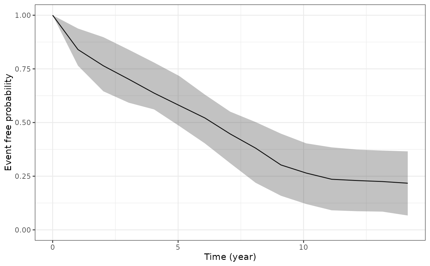
  # Lastly, if we wanted to obtain "standardised" survival probabilities,
  # (by averaging over the observed distribution of the fixed effect
  # covariates, as well as averaging over the estimated random effects
  # for individuals in our estimation sample or new data) then we can
  # specify 'standardise = TRUE'. We can then plot the resulting
  # standardised survival curve.
  ps4 <- posterior_survfit(example_jm, standardise = TRUE,
                           times = 0, extrapolate = TRUE)
  plot(ps4)
# }
}
#> Drawing new random effects for 2 individuals. Monitoring progress:
#> 
  |                                                                            
  |                                                                      |   0%
  |                                                                            
  |===================================                                   |  50%
  |                                                                            
  |======================================================================| 100%