Plot the estimated subject-specific or marginal survival function

This generic plot method for survfit.stanjm objects will plot the estimated subject-specific or marginal survival function using the data frame returned by a call to posterior_survfit. The call to posterior_survfit should ideally have included an "extrapolation" of the survival function, obtained by setting the extrapolate argument to TRUE.

The plot_stack_jm function takes arguments containing the plots of the estimated subject-specific longitudinal trajectory (or trajectories if a multivariate joint model was estimated) and the plot of the estimated subject-specific survival function and combines them into a single figure. This is most easily understood by running the Examples below.

Usage

# S3 method for class 'survfit.stanjm'
plot(
  x,
  ids = NULL,
  limits = c("ci", "none"),
  xlab = NULL,
  ylab = NULL,
  facet_scales = "free",
  ci_geom_args = NULL,
  ...
)

plot_stack_jm(yplot, survplot)

Arguments

x: A data frame and object of class survfit.stanjm returned by a call to the function posterior_survfit. The object contains point estimates and uncertainty interval limits for estimated values of the survival function.
ids: An optional vector providing a subset of subject IDs for whom the predicted curves should be plotted.
limits: A quoted character string specifying the type of limits to include in the plot. Can be one of: "ci" for the Bayesian posterior uncertainty interval for the estimated survival probability (often known as a credible interval); or "none" for no interval limits.
xlab, ylab: An optional axis label passed to labs.
facet_scales: A character string passed to the scales argument of facet_wrap when plotting the longitudinal trajectory for more than one individual.
ci_geom_args: Optional arguments passed to geom_ribbon and used to control features of the plotted interval limits. They should be supplied as a named list.
...: Optional arguments passed to geom_line and used to control features of the plotted survival function.
yplot: An object of class plot.predict.stanjm, returned by a call to the generic plot method for objects of class predict.stanjm. If there is more than one longitudinal outcome, then a list of such objects can be provided.
survplot: An object of class plot.survfit.stanjm, returned by a call to the generic plot method for objects of class survfit.stanjm.

Value

The plot method returns a ggplot object, also of class plot.survfit.stanjm. This object can be further customised using the ggplot2 package. It can also be passed to the function plot_stack_jm.

plot_stack_jm returns an object of class bayesplot_grid that includes plots of the estimated subject-specific longitudinal trajectories stacked on top of the associated subject-specific survival curve.

Examples

if (.Platform$OS.type != "windows" || .Platform$r_arch != "i386") {
# \donttest{
  # Run example model if not already loaded
  if (!exists("example_jm")) example(example_jm)

  # Obtain subject-specific conditional survival probabilities
  # for all individuals in the estimation dataset.
  ps1 <- posterior_survfit(example_jm, extrapolate = TRUE)

  # We then plot the conditional survival probabilities for
  # a subset of individuals
  plot(ps1, ids = c(7,13,15))
  # We can change or add attributes to the plot
  plot(ps1, ids = c(7,13,15), limits = "none")
  plot(ps1, ids = c(7,13,15), xlab = "Follow up time")
  plot(ps1, ids = c(7,13,15), ci_geom_args = list(fill = "red"),
       color = "blue", linetype = 2)
  plot(ps1, ids = c(7,13,15), facet_scales = "fixed")

  # Since the returned plot is also a ggplot object, we can
  # modify some of its attributes after it has been returned
  plot1 <- plot(ps1, ids = c(7,13,15))
  plot1 +
    ggplot2::theme(strip.background = ggplot2::element_blank()) +
    ggplot2::coord_cartesian(xlim = c(0, 15)) +
    ggplot2::labs(title = "Some plotted survival functions")

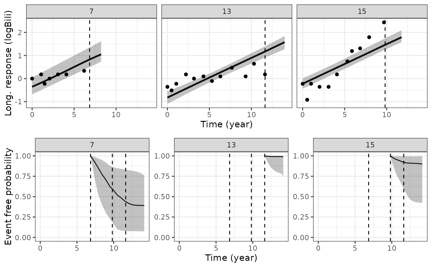
  # We can also combine the plot(s) of the estimated
  # subject-specific survival functions, with plot(s)
  # of the estimated longitudinal trajectories for the
  # same individuals
  ps1 <- posterior_survfit(example_jm, ids = c(7,13,15))
  pt1 <- posterior_traj(example_jm, , ids = c(7,13,15))
  plot_surv <- plot(ps1)
  plot_traj <- plot(pt1, vline = TRUE, plot_observed = TRUE)
  plot_stack_jm(plot_traj, plot_surv)

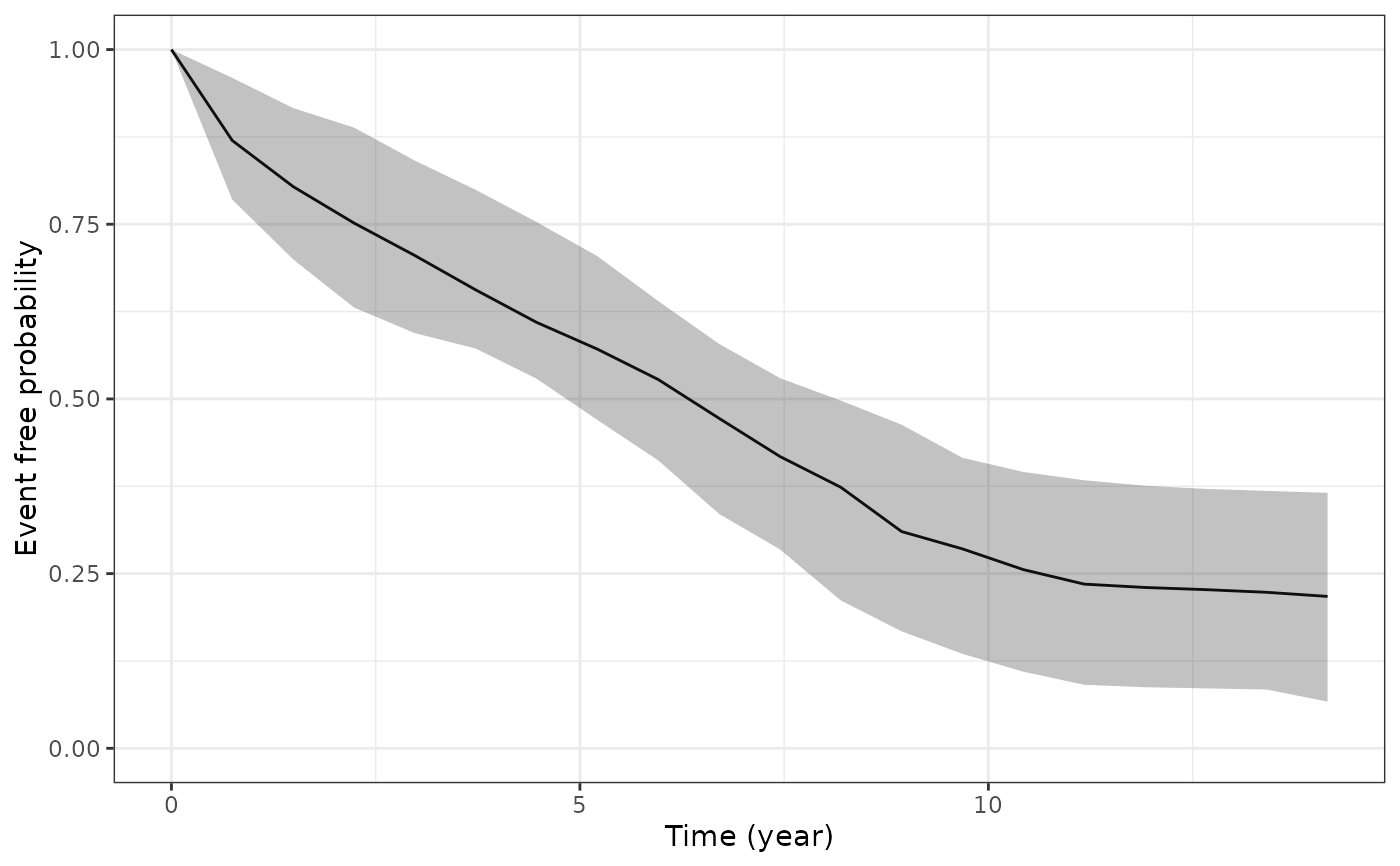
  # Lastly, let us plot the standardised survival function
  # based on all individuals in our estimation dataset
  ps2 <- posterior_survfit(example_jm, standardise = TRUE, times = 0,
                          control = list(epoints = 20))
  plot(ps2)
# }
}
#> Coordinate system already present.
#> ℹ Adding new coordinate system, which will replace the existing one.
#> `geom_smooth()` using formula = 'y ~ x'
#> `geom_smooth()` using formula = 'y ~ x'
#> `geom_smooth()` using formula = 'y ~ x'
#> `geom_smooth()` using formula = 'y ~ x'

if (.Platform$OS.type != "windows" || .Platform$r_arch != "i386") {
# \donttest{
  if (!exists("example_jm")) example(example_jm)
  ps1 <- posterior_survfit(example_jm, ids = c(7,13,15))
  pt1 <- posterior_traj(example_jm, ids = c(7,13,15), extrapolate = TRUE)
  plot_surv <- plot(ps1)
  plot_traj <- plot(pt1, vline = TRUE, plot_observed = TRUE)
  plot_stack_jm(plot_traj, plot_surv)
# }
}
#> `geom_smooth()` using formula = 'y ~ x'
#> `geom_smooth()` using formula = 'y ~ x'
#> `geom_smooth()` using formula = 'y ~ x'
#> `geom_smooth()` using formula = 'y ~ x'

Plot the estimated subject-specific or marginal survival function

Usage

Arguments

Value

See also

Examples