Markov chain traceplots

Draw the traceplot corresponding to one or more Markov chains, providing a visual way to inspect sampling behavior and assess mixing across chains and convergence.

<!-- %% traceplot(object, \dots)   -->
  # S4 method for stanfit
traceplot(object, pars, include = TRUE, unconstrain = FALSE, 
          inc_warmup = FALSE, window = NULL, nrow = NULL, ncol = NULL, ...)

Methods

traceplot

signature(object = "stanfit")

Plot the sampling paths for all chains.

Arguments

object

An instance of class stanfit.

pars

A character vector of parameter names. Defaults to all parameters or the first 10 parameters (if there are more than 10).

include

Should the parameters given by the pars argument be included (the default) or excluded from the plot? Only relevant if pars is not missing.

inc_warmup

TRUE or FALSE, indicating whether the warmup sample are included in the trace plot; defaults to FALSE.

window

A vector of length 2. Iterations between window[1] and window[2] will be shown in the plot. The default is to show all iterations if inc_warmup is TRUE and all iterations from the sampling period only if inc_warmup is FALSE. If inc_warmup is FALSE the iterations specified in window should not include iterations from the warmup period.

unconstrain

Should parameters be plotted on the unconstrained space? Defaults to FALSE.

nrow,ncol

Passed to facet_wrap.

...

Optional arguments to pass to geom_path (e.g. size, linetype, alpha, etc.).

Value

A ggplot object that can be further customized using the ggplot2 package.

See also

List of RStan plotting functions, Plot options

Examples

if (FALSE) {
# Create a stanfit object from reading CSV files of samples (saved in rstan
# package) generated by funtion stan for demonstration purpose from model as follows. 
# 
excode <- '
  transformed data {
    real y[20];
    y[1] <- 0.5796;  y[2]  <- 0.2276;   y[3] <- -0.2959; 
    y[4] <- -0.3742; y[5]  <- 0.3885;   y[6] <- -2.1585;
    y[7] <- 0.7111;  y[8]  <- 1.4424;   y[9] <- 2.5430; 
    y[10] <- 0.3746; y[11] <- 0.4773;   y[12] <- 0.1803; 
    y[13] <- 0.5215; y[14] <- -1.6044;  y[15] <- -0.6703; 
    y[16] <- 0.9459; y[17] <- -0.382;   y[18] <- 0.7619;
    y[19] <- 0.1006; y[20] <- -1.7461;
  }
  parameters {
    real mu;
    real<lower=0, upper=10> sigma;
    vector[2] z[3];
    real<lower=0> alpha;
  } 
  model {
    y ~ normal(mu, sigma);
    for (i in 1:3) 
      z[i] ~ normal(0, 1);
    alpha ~ exponential(2);
  } 
'
# exfit <- stan(model_code = excode, save_dso = FALSE, iter = 200, 
#               sample_file = "rstan_doc_ex.csv")
# 
exfit <- read_stan_csv(dir(system.file('misc', package = 'rstan'),
                       pattern='rstan_doc_ex_[[:digit:]].csv',
                       full.names = TRUE))

print(exfit)
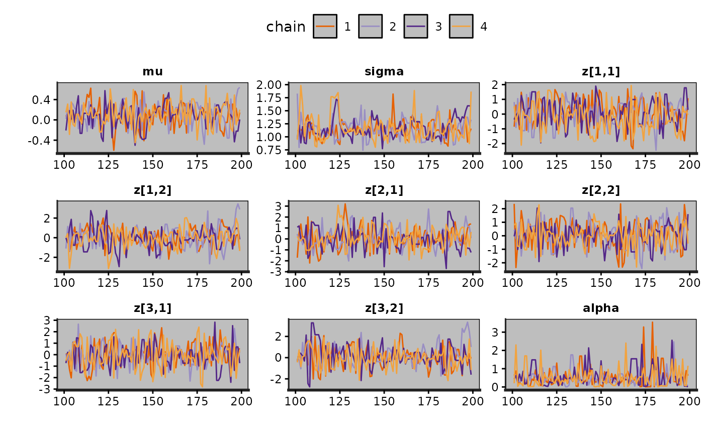
traceplot(exfit)
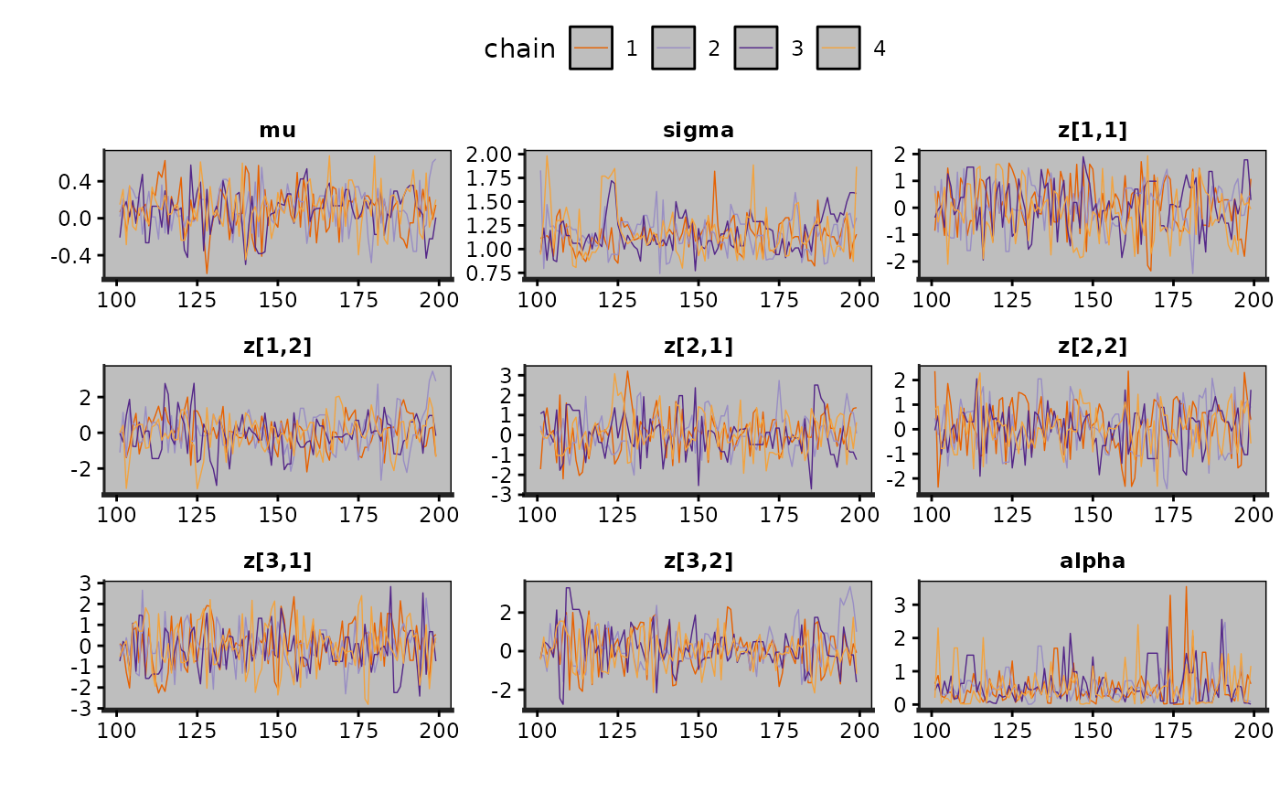
traceplot(exfit, size = 0.25)
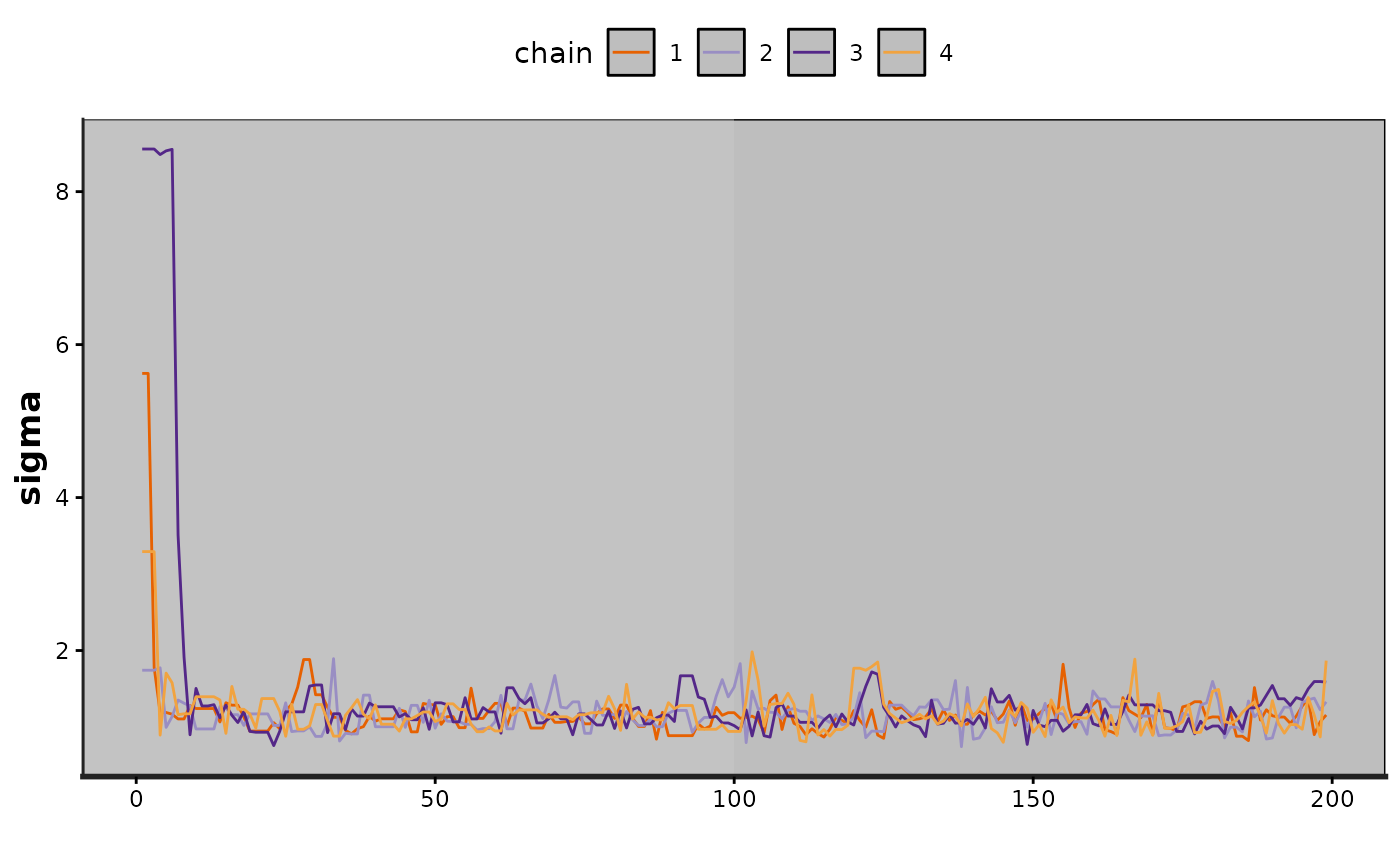
traceplot(exfit, pars = "sigma", inc_warmup = TRUE)

trace <- traceplot(exfit, pars = c("z[1,1]", "z[3,1]"))
trace + scale_color_discrete() + theme(legend.position = "top")
}