Fit a model with Stan

Fit a model defined in the Stan modeling language and return the fitted result as an instance of stanfit.

Usage

stan(file, model_name = "anon_model", model_code = "", fit = NA,
  data = list(), pars = NA,
  chains = 4, iter = 2000, warmup = floor(iter/2), thin = 1,
  init = "random", seed = sample.int(.Machine$integer.max, 1),
  algorithm = c("NUTS", "HMC", "Fixed_param"), <!-- %, "Metropolis"), -->
  control = NULL, sample_file = NULL, diagnostic_file = NULL,
  save_dso = TRUE, verbose = FALSE, include = TRUE,
  cores = getOption("mc.cores", 1L),
  open_progress = interactive() && !isatty(stdout()) &&
                  !identical(Sys.getenv("RSTUDIO"), "1"),
  ...,
  boost_lib = NULL, eigen_lib = NULL
  )

Arguments

file

The path to the Stan program to use. file should be a character string file name or a connection that R supports containing the text of a model specification in the Stan modeling language.

A model may also be specified directly as a character string using the model_code argument, but we recommend always putting Stan programs in separate files with a .stan extension.

The stan function can also use the Stan program from an existing stanfit object via the fit argument. When fit is specified, the file argument is ignored.

model_code

A character string either containing the model definition or the name of a character string object in the workspace. This argument is used only if arguments file and fit are not specified.

fit

An instance of S4 class stanfit derived from a previous fit; defaults to NA. If fit is not NA, the compiled model associated with the fitted result is re-used; thus the time that would otherwise be spent recompiling the C++ code for the model can be saved.

model_name

A string to use as the name of the model; defaults to "anon_model". However, the model name will be derived from file or model_code (if model_code is the name of a character string object) if model_name is not specified. This is not a particularly important argument, although since it affects the name used in printed messages, developers of other packages that use rstan to fit models may want to use informative names.

data

A named list or environment providing the data for the model, or a character vector for all the names of objects to use as data. See the Passing data to Stan section below.

pars

A character vector specifying parameters of interest to be saved. The default is to save all parameters from the model. If include = TRUE, only samples for parameters named in pars are stored in the fitted results. Conversely, if include = FALSE, samples for all parameters except those named in pars are stored in the fitted results.

include

Logical scalar defaulting to TRUE indicating whether to include or exclude the parameters given by the pars argument. If FALSE, only entire multidimensional parameters can be excluded, rather than particular elements of them.

iter

A positive integer specifying the number of iterations for each chain (including warmup). The default is 2000.

warmup

A positive integer specifying the number of warmup (aka burnin) iterations per chain. If step-size adaptation is on (which it is by default), this also controls the number of iterations for which adaptation is run (and hence these warmup samples should not be used for inference). The number of warmup iterations should be smaller than iter and the default is iter/2.

chains

A positive integer specifying the number of Markov chains. The default is 4.

cores

The number of cores to use when executing the Markov chains in parallel. The default is to use the value of the "mc.cores" option if it has been set and otherwise to default to 1 core. However, we recommend setting it to be as many processors as the hardware and RAM allow (up to the number of chains). See detectCores if you don't know this number for your system.

thin

A positive integer specifying the period for saving samples. The default is 1, which is usually the recommended value. Unless your posterior distribution takes up too much memory we do not recommend thinning as it throws away information. The tradition of thinning when running MCMC stems primarily from the use of samplers that require a large number of iterations to achieve the desired effective sample size. Because of the efficiency (effective samples per second) of Hamiltonian Monte Carlo, rarely should this be necessary when using Stan.

init

Specification of initial values for all or some parameters. Can be the digit 0, the strings "0" or "random", a function that returns a named list, or a list of named lists:

init="random" (default):

Let Stan generate random initial values for all parameters. The seed of the random number generator used by Stan can be specified via the seed argument. If the seed for Stan is fixed, the same initial values are used. The default is to randomly generate initial values between -2 and 2 on the unconstrained support. The optional additional parameter init_r can be set to some value other than 2 to change the range of the randomly generated inits.

init="0", init=0:

Initialize all parameters to zero on the unconstrained support.

inits via list:

Set inital values by providing a list equal in length to the number of chains. The elements of this list should themselves be named lists, where each of these named lists has the name of a parameter and is used to specify the initial values for that parameter for the corresponding chain.

inits via function:

Set initial values by providing a function that returns a list for specifying the initial values of parameters for a chain. The function can take an optional parameter chain_id through which the chain_id (if specified) or the integers from 1 to chains will be supplied to the function for generating initial values. See the Examples section below for examples of defining such functions and using a list of lists for specifying initial values.

When specifying initial values via a list or function, any parameters for which values are not specified will receive initial values generated as described in the init="random" description above.

seed

The seed for random number generation. The default is generated from 1 to the maximum integer supported by R on the machine. Even if multiple chains are used, only one seed is needed, with other chains having seeds derived from that of the first chain to avoid dependent samples. When a seed is specified by a number, as.integer will be applied to it. If as.integer produces NA, the seed is generated randomly. The seed can also be specified as a character string of digits, such as "12345", which is converted to integer.

Using R's set.seed function to set the seed for Stan will not work.

algorithm

One of the sampling algorithms that are implemented in Stan. The default and preferred algorithm is "NUTS", which is the No-U-Turn sampler variant of Hamiltonian Monte Carlo (Hoffman and Gelman 2011, Betancourt 2017). Currently the other options are "HMC" (Hamiltonian Monte Carlo), and "Fixed_param". When "Fixed_param" is used no MCMC sampling is performed (e.g., for simulating with in the generated quantities block).

sample_file

An optional character string providing the name of a file. If specified the draws for all parameters and other saved quantities will be written to the file. If not provided, files are not created. When the folder specified is not writable, tempdir() is used. When there are multiple chains, an underscore and chain number are appended to the file name.

diagnostic_file

An optional character string providing the name of a file. If specified the diagnostics data for all parameters will be written to the file. If not provided, files are not created. When the folder specified is not writable, tempdir() is used. When there are multiple chains, an underscore and chain number are appended to the file name.

save_dso

Logical, with default TRUE, indicating whether the dynamic shared object (DSO) compiled from the C++ code for the model will be saved or not. If TRUE, we can draw samples from the same model in another R session using the saved DSO (i.e., without compiling the C++ code again). This parameter only takes effect if fit is not used; with fit defined, the DSO from the previous run is used. When save_dso=TRUE, the fitted object can be loaded from what is saved previously and used for sampling, if the compiling is done on the same platform, that is, same operating system and same architecture (32bits or 64bits).

verbose

TRUE or FALSE: flag indicating whether to print intermediate output from Stan on the console, which might be helpful for model debugging.

control

A named list of parameters to control the sampler's behavior. It defaults to NULL so all the default values are used. First, the following are adaptation parameters for sampling algorithms. These are parameters used in Stan with similar names here.

• adapt_engaged (logical)

• adapt_gamma (double, positive, defaults to 0.05)

• adapt_delta (double, between 0 and 1, defaults to 0.8)

• adapt_kappa (double, positive, defaults to 0.75)

• adapt_t0 (double, positive, defaults to 10)

• adapt_init_buffer (integer, positive, defaults to 75)

• adapt_term_buffer (integer, positive, defaults to 50)

• adapt_window (integer, positive, defaults to 25)

In addition, algorithm HMC (called 'static HMC' in Stan) and NUTS share the following parameters:

• stepsize (double, positive, defaults to 1) Note: this controls the initial stepsize only, unless adapt_engaged=FALSE.

• stepsize_jitter (double, [0,1], defaults to 0)

• metric (string, one of "unit_e", "diag_e", "dense_e", defaults to "diag_e")

For algorithm NUTS, we can also set:

• max_treedepth (integer, positive, defaults to 10)

For algorithm HMC, we can also set:

• int_time (double, positive)

For test_grad mode, the following parameters can be set:

• epsilon (double, defaults to 1e-6)

• error (double, defaults to 1e-6)

open_progress

Logical scalar that only takes effect if cores > 1 but is recommended to be TRUE in interactive use so that the progress of the chains will be redirected to a file that is automatically opened for inspection. For very short runs, the user might prefer FALSE.

...

Other optional parameters:

• chain_id (integer)

• init_r (double, positive)

• test_grad (logical)

• append_samples (logical)

• refresh(integer)

• save_warmup(logical)

• deprecated: enable_random_init(logical)

chain_id can be a vector to specify the chain_id for all chains or an integer. For the former case, they should be unique. For the latter, the sequence of integers starting from the given chain_id are used for all chains.

init_r is used only for generating random initial values, specifically when init="random" or not all parameters are initialized in the user-supplied list or function. If specified, the initial values are simulated uniformly from interval [-init_r, init_r] rather than using the default interval (see the manual of (cmd)Stan).

test_grad (logical). If test_grad=TRUE, Stan will not do any sampling. Instead, the gradient calculation is tested and printed out and the fitted stanfit object is in test gradient mode. By default, it is FALSE.

append_samples (logical). Only relevant if sample_file is specified and is an existing file. In that case, setting append_samples=TRUE will append the samples to the existing file rather than overwriting the contents of the file.

refresh (integer) can be used to control how often the progress of the sampling is reported (i.e. show the progress every refresh iterations). By default, refresh = max(iter/10, 1). The progress indicator is turned off if refresh <= 0.

Deprecated: enable_random_init (logical) being TRUE enables specifying initial values randomly when the initial values are not fully specified from the user.

save_warmup (logical) indicates whether to save draws during the warmup phase and defaults to TRUE. Some memory related problems can be avoided by setting it to FALSE, but some diagnostics are more limited if the warmup draws are not stored.

boost_lib

The path for an alternative version of the Boost C++ to use instead of the one in the BH package.

eigen_lib

The path for an alternative version of the Eigen C++ library to the one in RcppEigen.

Details

The stan function does all of the work of fitting a Stan model and returning the results as an instance of stanfit. The steps are roughly as follows:

1. Translate the Stan model to C++ code. (stanc)

2. Compile the C++ code into a binary shared object, which is loaded into the current R session (an object of S4 class stanmodel is created). (stan_model)

3. Draw samples and wrap them in an object of S4 class stanfit. (sampling)

The returned object can be used with methods such as print, summary, and plot to inspect and retrieve the results of the fitted model.

stan can also be used to sample again from a fitted model under different settings (e.g., different iter, data, etc.) by using the fit argument to specify an existing stanfit object. In this case, the compiled C++ code for the model is reused.

Value

An object of S4 class stanfit. However, if cores > 1 and there is an error for any of the chains, then the error(s) are printed. If all chains have errors and an error occurs before or during sampling, the returned object does not contain samples. But the compiled binary object for the model is still included, so we can reuse the returned object for another sampling.

Passing data to Stan

The data passed to stan are preprocessed before being passed to Stan. If data is not a character vector, the data block of the Stan program is parsed and R objects of the same name are searched starting from the calling environment. Then, if data is list-like but not a data.frame the elements of data take precedence. This behavior is similar to how a formula is evaluated by the lm function when data is supplied. In general, each R object being passed to Stan should be either a numeric vector (including the special case of a 'scalar') or a numeric array (matrix). The first exception is that an element can be a logical vector: TRUE's are converted to 1 and FALSE's to 0. An element can also be a data frame or a specially structured list (see details below), both of which will be converted into arrays in the preprocessing. Using a specially structured list is not encouraged though it might be convenient sometimes; and when in doubt, just use arrays.

This preprocessing for each element mainly includes the following:

1. Change the data of type from double to integer if no accuracy is lost. The main reason is that by default, R uses double as data type such as in a <- 3. But Stan will not read data of type int from real and it reads data from int if the data type is declared as real.

2. Check if there is NA in the data. Unlike BUGS, Stan does not allow missing data. Any NA values in supplied data will cause the function to stop and report an error.

3. Check data types. Stan allows only numeric data, that is, doubles, integers, and arrays of these. Data of other types (for example, characters and factors) are not passed to Stan.

4. Check whether there are objects in the data list with duplicated names. Duplicated names, if found, will cause the function to stop and report an error.

5. Check whether the names of objects in the data list are legal Stan names. If illegal names are found, it will stop and report an error. See (Cmd)Stan's manual for the rules of variable names.

6. When an element is of type data.frame, it will be converted to matrix by function data.matrix.

7. When an element is of type list, it is supposed to make it easier to pass data for those declared in Stan code such as "vector[J] y1[I]" and "matrix[J,K] y2[I]". Using the latter as an example, we can use a list for y2 if the list has "I" elements, each of which is an array (matrix) of dimension "J*K". However, it is not possible to pass a list for data declared such as "vector[K] y3[I,J]"; the only way for it is to use an array with dimension "I*J*K". In addition, technically a data.frame in R is also a list, but it should not be used for the purpose here since a data.frame will be converted to a matrix as described above.

Stan treats a vector of length 1 in R as a scalar. So technically if, for example, "array[1] real y;" is defined in the data block, an array such as "y = array(1.0, dim = 1)" in R should be used. This is also the case for specifying initial values since the same underlying approach for reading data from R in Stan is used, in which vector of length 1 is treated as a scalar.

In general, the higher the optimization level is set, the faster the generated binary code for the model runs, which can be set in a Makevars file. However, the binary code generated for the model runs fast by using a higher optimization level at the cost of longer times to compile the C++ code.

References

The Stan Development Team Stan Modeling Language User's Guide and Reference Manual. https://mc-stan.org.

The Stan Development Team CmdStan Interface User's Guide. https://mc-stan.org.

See also

• The package vignettes for an example of fitting a model and accessing the contents of stanfit objects (https://mc-stan.org/rstan/articles/).

• stanc for translating model code in Stan modeling language to C++, sampling for sampling, and stanfit for the fitted results.

• as.array.stanfit and extract for extracting samples from stanfit objects.

Examples

# \dontrun{
#### example 1
library(rstan)
scode <- "
parameters {
  array[2] real y;
}
model {
  y[1] ~ normal(0, 1);
  y[2] ~ double_exponential(0, 2);
}
"
fit1 <- stan(model_code = scode, iter = 10, verbose = FALSE)
#> 
#> SAMPLING FOR MODEL 'anon_model' NOW (CHAIN 1).
#> Chain 1: 
#> Chain 1: Gradient evaluation took 2e-06 seconds
#> Chain 1: 1000 transitions using 10 leapfrog steps per transition would take 0.02 seconds.
#> Chain 1: Adjust your expectations accordingly!
#> Chain 1: 
#> Chain 1: 
#> Chain 1: WARNING: No variance estimation is
#> Chain 1:          performed for num_warmup < 20
#> Chain 1: 
#> Chain 1: Iteration: 1 / 10 [ 10%]  (Warmup)
#> Chain 1: Iteration: 2 / 10 [ 20%]  (Warmup)
#> Chain 1: Iteration: 3 / 10 [ 30%]  (Warmup)
#> Chain 1: Iteration: 4 / 10 [ 40%]  (Warmup)
#> Chain 1: Iteration: 5 / 10 [ 50%]  (Warmup)
#> Chain 1: Iteration: 6 / 10 [ 60%]  (Sampling)
#> Chain 1: Iteration: 7 / 10 [ 70%]  (Sampling)
#> Chain 1: Iteration: 8 / 10 [ 80%]  (Sampling)
#> Chain 1: Iteration: 9 / 10 [ 90%]  (Sampling)
#> Chain 1: Iteration: 10 / 10 [100%]  (Sampling)
#> Chain 1: 
#> Chain 1:  Elapsed Time: 0 seconds (Warm-up)
#> Chain 1:                0 seconds (Sampling)
#> Chain 1:                0 seconds (Total)
#> Chain 1: 
#> 
#> SAMPLING FOR MODEL 'anon_model' NOW (CHAIN 2).
#> Chain 2: 
#> Chain 2: Gradient evaluation took 1e-06 seconds
#> Chain 2: 1000 transitions using 10 leapfrog steps per transition would take 0.01 seconds.
#> Chain 2: Adjust your expectations accordingly!
#> Chain 2: 
#> Chain 2: 
#> Chain 2: WARNING: No variance estimation is
#> Chain 2:          performed for num_warmup < 20
#> Chain 2: 
#> Chain 2: Iteration: 1 / 10 [ 10%]  (Warmup)
#> Chain 2: Iteration: 2 / 10 [ 20%]  (Warmup)
#> Chain 2: Iteration: 3 / 10 [ 30%]  (Warmup)
#> Chain 2: Iteration: 4 / 10 [ 40%]  (Warmup)
#> Chain 2: Iteration: 5 / 10 [ 50%]  (Warmup)
#> Chain 2: Iteration: 6 / 10 [ 60%]  (Sampling)
#> Chain 2: Iteration: 7 / 10 [ 70%]  (Sampling)
#> Chain 2: Iteration: 8 / 10 [ 80%]  (Sampling)
#> Chain 2: Iteration: 9 / 10 [ 90%]  (Sampling)
#> Chain 2: Iteration: 10 / 10 [100%]  (Sampling)
#> Chain 2: 
#> Chain 2:  Elapsed Time: 0 seconds (Warm-up)
#> Chain 2:                0 seconds (Sampling)
#> Chain 2:                0 seconds (Total)
#> Chain 2: 
#> 
#> SAMPLING FOR MODEL 'anon_model' NOW (CHAIN 3).
#> Chain 3: 
#> Chain 3: Gradient evaluation took 1e-06 seconds
#> Chain 3: 1000 transitions using 10 leapfrog steps per transition would take 0.01 seconds.
#> Chain 3: Adjust your expectations accordingly!
#> Chain 3: 
#> Chain 3: 
#> Chain 3: WARNING: No variance estimation is
#> Chain 3:          performed for num_warmup < 20
#> Chain 3: 
#> Chain 3: Iteration: 1 / 10 [ 10%]  (Warmup)
#> Chain 3: Iteration: 2 / 10 [ 20%]  (Warmup)
#> Chain 3: Iteration: 3 / 10 [ 30%]  (Warmup)
#> Chain 3: Iteration: 4 / 10 [ 40%]  (Warmup)
#> Chain 3: Iteration: 5 / 10 [ 50%]  (Warmup)
#> Chain 3: Iteration: 6 / 10 [ 60%]  (Sampling)
#> Chain 3: Iteration: 7 / 10 [ 70%]  (Sampling)
#> Chain 3: Iteration: 8 / 10 [ 80%]  (Sampling)
#> Chain 3: Iteration: 9 / 10 [ 90%]  (Sampling)
#> Chain 3: Iteration: 10 / 10 [100%]  (Sampling)
#> Chain 3: 
#> Chain 3:  Elapsed Time: 0 seconds (Warm-up)
#> Chain 3:                0 seconds (Sampling)
#> Chain 3:                0 seconds (Total)
#> Chain 3: 
#> 
#> SAMPLING FOR MODEL 'anon_model' NOW (CHAIN 4).
#> Chain 4: 
#> Chain 4: Gradient evaluation took 1e-06 seconds
#> Chain 4: 1000 transitions using 10 leapfrog steps per transition would take 0.01 seconds.
#> Chain 4: Adjust your expectations accordingly!
#> Chain 4: 
#> Chain 4: 
#> Chain 4: WARNING: No variance estimation is
#> Chain 4:          performed for num_warmup < 20
#> Chain 4: 
#> Chain 4: Iteration: 1 / 10 [ 10%]  (Warmup)
#> Chain 4: Iteration: 2 / 10 [ 20%]  (Warmup)
#> Chain 4: Iteration: 3 / 10 [ 30%]  (Warmup)
#> Chain 4: Iteration: 4 / 10 [ 40%]  (Warmup)
#> Chain 4: Iteration: 5 / 10 [ 50%]  (Warmup)
#> Chain 4: Iteration: 6 / 10 [ 60%]  (Sampling)
#> Chain 4: Iteration: 7 / 10 [ 70%]  (Sampling)
#> Chain 4: Iteration: 8 / 10 [ 80%]  (Sampling)
#> Chain 4: Iteration: 9 / 10 [ 90%]  (Sampling)
#> Chain 4: Iteration: 10 / 10 [100%]  (Sampling)
#> Chain 4: 
#> Chain 4:  Elapsed Time: 0 seconds (Warm-up)
#> Chain 4:                0 seconds (Sampling)
#> Chain 4:                0 seconds (Total)
#> Chain 4: 
#> Warning: The largest R-hat is 1.95, indicating chains have not mixed.
#> Running the chains for more iterations may help. See
#> https://mc-stan.org/misc/warnings.html#r-hat
print(fit1)
#> Inference for Stan model: anon_model.
#> 4 chains, each with iter=10; warmup=5; thin=1; 
#> post-warmup draws per chain=5, total post-warmup draws=20.
#> 
#>       mean se_mean   sd  2.5%   25%   50%   75% 97.5% n_eff Rhat
#> y[1]  0.22    0.34 0.97 -1.66 -0.16  0.13  0.75  1.80     8 1.72
#> y[2] -1.53    1.15 2.50 -4.90 -3.48 -1.78 -0.52  3.57     5 2.04
#> lp__ -1.71    0.24 0.94 -3.15 -2.40 -1.87 -0.87 -0.33    16 1.02
#> 
#> Samples were drawn using NUTS(diag_e) at Wed Dec 10 00:21:08 2025.
#> For each parameter, n_eff is a crude measure of effective sample size,
#> and Rhat is the potential scale reduction factor on split chains (at 
#> convergence, Rhat=1).
fit2 <- stan(fit = fit1, iter = 10000, verbose = FALSE)
#> 
#> SAMPLING FOR MODEL 'anon_model' NOW (CHAIN 1).
#> Chain 1: 
#> Chain 1: Gradient evaluation took 2e-06 seconds
#> Chain 1: 1000 transitions using 10 leapfrog steps per transition would take 0.02 seconds.
#> Chain 1: Adjust your expectations accordingly!
#> Chain 1: 
#> Chain 1: 
#> Chain 1: Iteration:    1 / 10000 [  0%]  (Warmup)
#> Chain 1: Iteration: 1000 / 10000 [ 10%]  (Warmup)
#> Chain 1: Iteration: 2000 / 10000 [ 20%]  (Warmup)
#> Chain 1: Iteration: 3000 / 10000 [ 30%]  (Warmup)
#> Chain 1: Iteration: 4000 / 10000 [ 40%]  (Warmup)
#> Chain 1: Iteration: 5000 / 10000 [ 50%]  (Warmup)
#> Chain 1: Iteration: 5001 / 10000 [ 50%]  (Sampling)
#> Chain 1: Iteration: 6000 / 10000 [ 60%]  (Sampling)
#> Chain 1: Iteration: 7000 / 10000 [ 70%]  (Sampling)
#> Chain 1: Iteration: 8000 / 10000 [ 80%]  (Sampling)
#> Chain 1: Iteration: 9000 / 10000 [ 90%]  (Sampling)
#> Chain 1: Iteration: 10000 / 10000 [100%]  (Sampling)
#> Chain 1: 
#> Chain 1:  Elapsed Time: 0.027 seconds (Warm-up)
#> Chain 1:                0.028 seconds (Sampling)
#> Chain 1:                0.055 seconds (Total)
#> Chain 1: 
#> 
#> SAMPLING FOR MODEL 'anon_model' NOW (CHAIN 2).
#> Chain 2: 
#> Chain 2: Gradient evaluation took 1e-06 seconds
#> Chain 2: 1000 transitions using 10 leapfrog steps per transition would take 0.01 seconds.
#> Chain 2: Adjust your expectations accordingly!
#> Chain 2: 
#> Chain 2: 
#> Chain 2: Iteration:    1 / 10000 [  0%]  (Warmup)
#> Chain 2: Iteration: 1000 / 10000 [ 10%]  (Warmup)
#> Chain 2: Iteration: 2000 / 10000 [ 20%]  (Warmup)
#> Chain 2: Iteration: 3000 / 10000 [ 30%]  (Warmup)
#> Chain 2: Iteration: 4000 / 10000 [ 40%]  (Warmup)
#> Chain 2: Iteration: 5000 / 10000 [ 50%]  (Warmup)
#> Chain 2: Iteration: 5001 / 10000 [ 50%]  (Sampling)
#> Chain 2: Iteration: 6000 / 10000 [ 60%]  (Sampling)
#> Chain 2: Iteration: 7000 / 10000 [ 70%]  (Sampling)
#> Chain 2: Iteration: 8000 / 10000 [ 80%]  (Sampling)
#> Chain 2: Iteration: 9000 / 10000 [ 90%]  (Sampling)
#> Chain 2: Iteration: 10000 / 10000 [100%]  (Sampling)
#> Chain 2: 
#> Chain 2:  Elapsed Time: 0.026 seconds (Warm-up)
#> Chain 2:                0.025 seconds (Sampling)
#> Chain 2:                0.051 seconds (Total)
#> Chain 2: 
#> 
#> SAMPLING FOR MODEL 'anon_model' NOW (CHAIN 3).
#> Chain 3: 
#> Chain 3: Gradient evaluation took 1e-06 seconds
#> Chain 3: 1000 transitions using 10 leapfrog steps per transition would take 0.01 seconds.
#> Chain 3: Adjust your expectations accordingly!
#> Chain 3: 
#> Chain 3: 
#> Chain 3: Iteration:    1 / 10000 [  0%]  (Warmup)
#> Chain 3: Iteration: 1000 / 10000 [ 10%]  (Warmup)
#> Chain 3: Iteration: 2000 / 10000 [ 20%]  (Warmup)
#> Chain 3: Iteration: 3000 / 10000 [ 30%]  (Warmup)
#> Chain 3: Iteration: 4000 / 10000 [ 40%]  (Warmup)
#> Chain 3: Iteration: 5000 / 10000 [ 50%]  (Warmup)
#> Chain 3: Iteration: 5001 / 10000 [ 50%]  (Sampling)
#> Chain 3: Iteration: 6000 / 10000 [ 60%]  (Sampling)
#> Chain 3: Iteration: 7000 / 10000 [ 70%]  (Sampling)
#> Chain 3: Iteration: 8000 / 10000 [ 80%]  (Sampling)
#> Chain 3: Iteration: 9000 / 10000 [ 90%]  (Sampling)
#> Chain 3: Iteration: 10000 / 10000 [100%]  (Sampling)
#> Chain 3: 
#> Chain 3:  Elapsed Time: 0.027 seconds (Warm-up)
#> Chain 3:                0.026 seconds (Sampling)
#> Chain 3:                0.053 seconds (Total)
#> Chain 3: 
#> 
#> SAMPLING FOR MODEL 'anon_model' NOW (CHAIN 4).
#> Chain 4: 
#> Chain 4: Gradient evaluation took 1e-06 seconds
#> Chain 4: 1000 transitions using 10 leapfrog steps per transition would take 0.01 seconds.
#> Chain 4: Adjust your expectations accordingly!
#> Chain 4: 
#> Chain 4: 
#> Chain 4: Iteration:    1 / 10000 [  0%]  (Warmup)
#> Chain 4: Iteration: 1000 / 10000 [ 10%]  (Warmup)
#> Chain 4: Iteration: 2000 / 10000 [ 20%]  (Warmup)
#> Chain 4: Iteration: 3000 / 10000 [ 30%]  (Warmup)
#> Chain 4: Iteration: 4000 / 10000 [ 40%]  (Warmup)
#> Chain 4: Iteration: 5000 / 10000 [ 50%]  (Warmup)
#> Chain 4: Iteration: 5001 / 10000 [ 50%]  (Sampling)
#> Chain 4: Iteration: 6000 / 10000 [ 60%]  (Sampling)
#> Chain 4: Iteration: 7000 / 10000 [ 70%]  (Sampling)
#> Chain 4: Iteration: 8000 / 10000 [ 80%]  (Sampling)
#> Chain 4: Iteration: 9000 / 10000 [ 90%]  (Sampling)
#> Chain 4: Iteration: 10000 / 10000 [100%]  (Sampling)
#> Chain 4: 
#> Chain 4:  Elapsed Time: 0.027 seconds (Warm-up)
#> Chain 4:                0.026 seconds (Sampling)
#> Chain 4:                0.053 seconds (Total)
#> Chain 4: 

## using as.array on the stanfit object to get samples
a2 <- as.array(fit2)

## extract samples as a list of arrays
e2 <- extract(fit2, permuted = FALSE)

#### example 2
#### the result of this package is included in the package

excode <- '
  transformed data {
    array[20] real y;
    y[1] = 0.5796;  y[2] = 0.2276;   y[3]  = -0.2959;
    y[4] = -0.3742; y[5] = 0.3885;   y[6]  = -2.1585;
    y[7] = 0.7111;  y[8] = 1.4424;   y[9]  = 2.5430;
    y[10] = 0.3746; y[11] = 0.4773;  y[12] = 0.1803;
    y[13] = 0.5215; y[14] = -1.6044; y[15] = -0.6703;
    y[16] = 0.9459; y[17] = -0.382;  y[18] = 0.7619;
    y[19] = 0.1006; y[20] = -1.7461;
  }
  parameters {
    real mu;
    real<lower=0, upper=10> sigma;
    array[3] vector[2] z;
    real<lower=0> alpha;
  }
  model {
    y ~ normal(mu, sigma);
    for (i in 1:3)
      z[i] ~ normal(0, 1);
    alpha ~ exponential(2);
  }
'

exfit <- stan(model_code = excode, save_dso = FALSE, iter = 500)
#> 
#> SAMPLING FOR MODEL 'anon_model' NOW (CHAIN 1).
#> Chain 1: 
#> Chain 1: Gradient evaluation took 7e-06 seconds
#> Chain 1: 1000 transitions using 10 leapfrog steps per transition would take 0.07 seconds.
#> Chain 1: Adjust your expectations accordingly!
#> Chain 1: 
#> Chain 1: 
#> Chain 1: Iteration:   1 / 500 [  0%]  (Warmup)
#> Chain 1: Iteration:  50 / 500 [ 10%]  (Warmup)
#> Chain 1: Iteration: 100 / 500 [ 20%]  (Warmup)
#> Chain 1: Iteration: 150 / 500 [ 30%]  (Warmup)
#> Chain 1: Iteration: 200 / 500 [ 40%]  (Warmup)
#> Chain 1: Iteration: 250 / 500 [ 50%]  (Warmup)
#> Chain 1: Iteration: 251 / 500 [ 50%]  (Sampling)
#> Chain 1: Iteration: 300 / 500 [ 60%]  (Sampling)
#> Chain 1: Iteration: 350 / 500 [ 70%]  (Sampling)
#> Chain 1: Iteration: 400 / 500 [ 80%]  (Sampling)
#> Chain 1: Iteration: 450 / 500 [ 90%]  (Sampling)
#> Chain 1: Iteration: 500 / 500 [100%]  (Sampling)
#> Chain 1: 
#> Chain 1:  Elapsed Time: 0.008 seconds (Warm-up)
#> Chain 1:                0.003 seconds (Sampling)
#> Chain 1:                0.011 seconds (Total)
#> Chain 1: 
#> 
#> SAMPLING FOR MODEL 'anon_model' NOW (CHAIN 2).
#> Chain 2: 
#> Chain 2: Gradient evaluation took 2e-06 seconds
#> Chain 2: 1000 transitions using 10 leapfrog steps per transition would take 0.02 seconds.
#> Chain 2: Adjust your expectations accordingly!
#> Chain 2: 
#> Chain 2: 
#> Chain 2: Iteration:   1 / 500 [  0%]  (Warmup)
#> Chain 2: Iteration:  50 / 500 [ 10%]  (Warmup)
#> Chain 2: Iteration: 100 / 500 [ 20%]  (Warmup)
#> Chain 2: Iteration: 150 / 500 [ 30%]  (Warmup)
#> Chain 2: Iteration: 200 / 500 [ 40%]  (Warmup)
#> Chain 2: Iteration: 250 / 500 [ 50%]  (Warmup)
#> Chain 2: Iteration: 251 / 500 [ 50%]  (Sampling)
#> Chain 2: Iteration: 300 / 500 [ 60%]  (Sampling)
#> Chain 2: Iteration: 350 / 500 [ 70%]  (Sampling)
#> Chain 2: Iteration: 400 / 500 [ 80%]  (Sampling)
#> Chain 2: Iteration: 450 / 500 [ 90%]  (Sampling)
#> Chain 2: Iteration: 500 / 500 [100%]  (Sampling)
#> Chain 2: 
#> Chain 2:  Elapsed Time: 0.008 seconds (Warm-up)
#> Chain 2:                0.003 seconds (Sampling)
#> Chain 2:                0.011 seconds (Total)
#> Chain 2: 
#> 
#> SAMPLING FOR MODEL 'anon_model' NOW (CHAIN 3).
#> Chain 3: 
#> Chain 3: Gradient evaluation took 3e-06 seconds
#> Chain 3: 1000 transitions using 10 leapfrog steps per transition would take 0.03 seconds.
#> Chain 3: Adjust your expectations accordingly!
#> Chain 3: 
#> Chain 3: 
#> Chain 3: Iteration:   1 / 500 [  0%]  (Warmup)
#> Chain 3: Iteration:  50 / 500 [ 10%]  (Warmup)
#> Chain 3: Iteration: 100 / 500 [ 20%]  (Warmup)
#> Chain 3: Iteration: 150 / 500 [ 30%]  (Warmup)
#> Chain 3: Iteration: 200 / 500 [ 40%]  (Warmup)
#> Chain 3: Iteration: 250 / 500 [ 50%]  (Warmup)
#> Chain 3: Iteration: 251 / 500 [ 50%]  (Sampling)
#> Chain 3: Iteration: 300 / 500 [ 60%]  (Sampling)
#> Chain 3: Iteration: 350 / 500 [ 70%]  (Sampling)
#> Chain 3: Iteration: 400 / 500 [ 80%]  (Sampling)
#> Chain 3: Iteration: 450 / 500 [ 90%]  (Sampling)
#> Chain 3: Iteration: 500 / 500 [100%]  (Sampling)
#> Chain 3: 
#> Chain 3:  Elapsed Time: 0.007 seconds (Warm-up)
#> Chain 3:                0.003 seconds (Sampling)
#> Chain 3:                0.01 seconds (Total)
#> Chain 3: 
#> 
#> SAMPLING FOR MODEL 'anon_model' NOW (CHAIN 4).
#> Chain 4: 
#> Chain 4: Gradient evaluation took 2e-06 seconds
#> Chain 4: 1000 transitions using 10 leapfrog steps per transition would take 0.02 seconds.
#> Chain 4: Adjust your expectations accordingly!
#> Chain 4: 
#> Chain 4: 
#> Chain 4: Iteration:   1 / 500 [  0%]  (Warmup)
#> Chain 4: Iteration:  50 / 500 [ 10%]  (Warmup)
#> Chain 4: Iteration: 100 / 500 [ 20%]  (Warmup)
#> Chain 4: Iteration: 150 / 500 [ 30%]  (Warmup)
#> Chain 4: Iteration: 200 / 500 [ 40%]  (Warmup)
#> Chain 4: Iteration: 250 / 500 [ 50%]  (Warmup)
#> Chain 4: Iteration: 251 / 500 [ 50%]  (Sampling)
#> Chain 4: Iteration: 300 / 500 [ 60%]  (Sampling)
#> Chain 4: Iteration: 350 / 500 [ 70%]  (Sampling)
#> Chain 4: Iteration: 400 / 500 [ 80%]  (Sampling)
#> Chain 4: Iteration: 450 / 500 [ 90%]  (Sampling)
#> Chain 4: Iteration: 500 / 500 [100%]  (Sampling)
#> Chain 4: 
#> Chain 4:  Elapsed Time: 0.008 seconds (Warm-up)
#> Chain 4:                0.003 seconds (Sampling)
#> Chain 4:                0.011 seconds (Total)
#> Chain 4: 
print(exfit)
#> Inference for Stan model: anon_model.
#> 4 chains, each with iter=500; warmup=250; thin=1; 
#> post-warmup draws per chain=250, total post-warmup draws=1000.
#> 
#>          mean se_mean   sd   2.5%    25%    50%    75%  97.5% n_eff Rhat
#> mu       0.11    0.01 0.28  -0.42  -0.08   0.11   0.30   0.65  1156 1.00
#> sigma    1.18    0.01 0.22   0.84   1.02   1.14   1.31   1.71  1138 1.00
#> z[1,1]  -0.02    0.02 0.97  -2.06  -0.66   0.01   0.67   1.87  2300 1.00
#> z[1,2]   0.01    0.02 1.03  -1.99  -0.67   0.00   0.65   2.02  1924 1.00
#> z[2,1]  -0.03    0.02 0.96  -1.86  -0.68  -0.05   0.65   1.83  1792 1.00
#> z[2,2]   0.01    0.02 1.02  -2.06  -0.67  -0.01   0.74   1.98  1816 1.00
#> z[3,1]   0.02    0.02 1.03  -1.98  -0.67   0.05   0.73   2.00  2861 1.00
#> z[3,2]   0.00    0.02 0.98  -1.94  -0.66   0.00   0.64   1.82  1832 1.00
#> alpha    0.50    0.01 0.54   0.01   0.15   0.34   0.66   1.88  1387 1.00
#> lp__   -17.76    0.11 2.30 -23.28 -18.95 -17.39 -16.12 -14.49   444 1.01
#> 
#> Samples were drawn using NUTS(diag_e) at Wed Dec 10 00:21:59 2025.
#> For each parameter, n_eff is a crude measure of effective sample size,
#> and Rhat is the potential scale reduction factor on split chains (at 
#> convergence, Rhat=1).
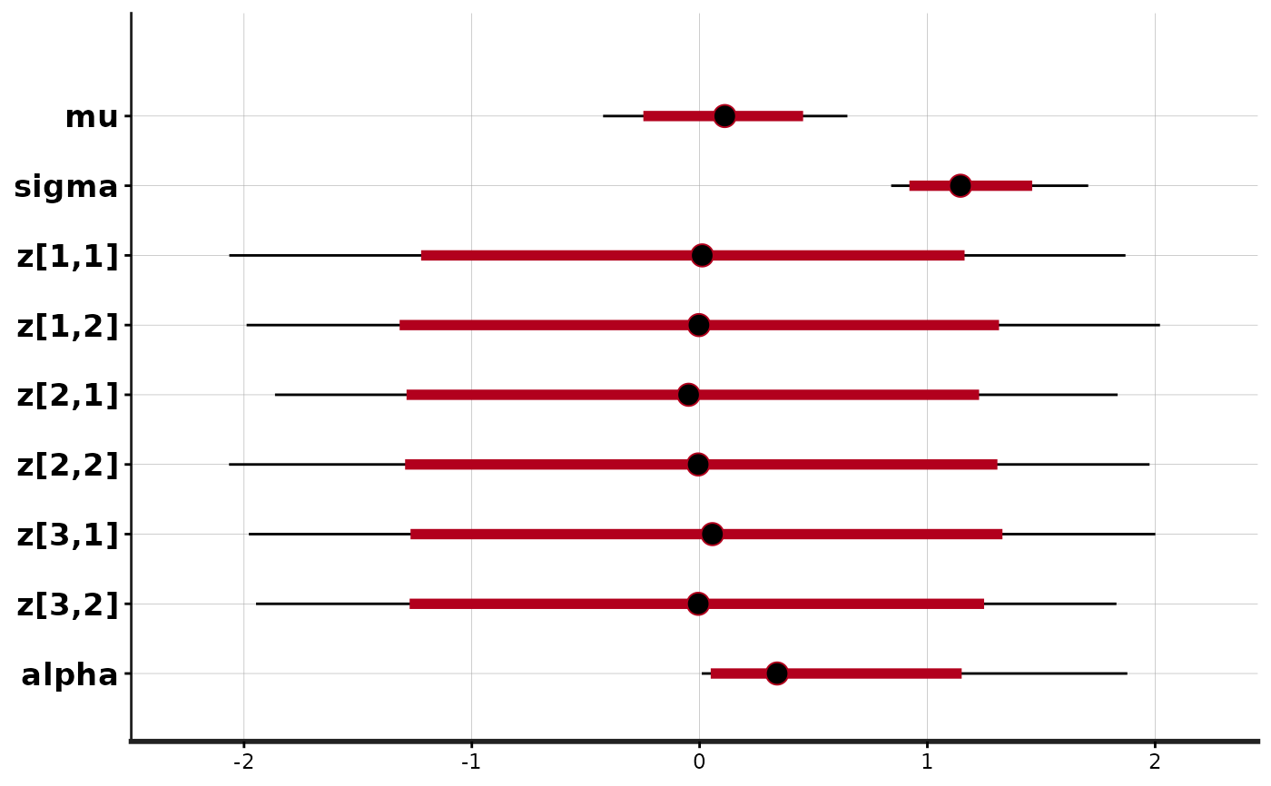
plot(exfit)
#> ci_level: 0.8 (80% intervals)
#> outer_level: 0.95 (95% intervals)

# }
# \dontrun{
## examples of specify argument `init` for function stan

## define a function to generate initial values that can
## be fed to function stan's argument `init`
# function form 1 without arguments
initf1 <- function() {
  list(mu = 1, sigma = 4, z = array(rnorm(6), dim = c(3,2)), alpha = 1)
}
# function form 2 with an argument named `chain_id`
initf2 <- function(chain_id = 1) {
  # cat("chain_id =", chain_id, "\n")
  list(mu = 1, sigma = 4, z = array(rnorm(6), dim = c(3,2)), alpha = chain_id)
}

# generate a list of lists to specify initial values
n_chains <- 4
init_ll <- lapply(1:n_chains, function(id) initf2(chain_id = id))

exfit0 <- stan(model_code = excode, init = initf1)
#> 
#> SAMPLING FOR MODEL 'anon_model' NOW (CHAIN 1).
#> Chain 1: 
#> Chain 1: Gradient evaluation took 7e-06 seconds
#> Chain 1: 1000 transitions using 10 leapfrog steps per transition would take 0.07 seconds.
#> Chain 1: Adjust your expectations accordingly!
#> Chain 1: 
#> Chain 1: 
#> Chain 1: Iteration:    1 / 2000 [  0%]  (Warmup)
#> Chain 1: Iteration:  200 / 2000 [ 10%]  (Warmup)
#> Chain 1: Iteration:  400 / 2000 [ 20%]  (Warmup)
#> Chain 1: Iteration:  600 / 2000 [ 30%]  (Warmup)
#> Chain 1: Iteration:  800 / 2000 [ 40%]  (Warmup)
#> Chain 1: Iteration: 1000 / 2000 [ 50%]  (Warmup)
#> Chain 1: Iteration: 1001 / 2000 [ 50%]  (Sampling)
#> Chain 1: Iteration: 1200 / 2000 [ 60%]  (Sampling)
#> Chain 1: Iteration: 1400 / 2000 [ 70%]  (Sampling)
#> Chain 1: Iteration: 1600 / 2000 [ 80%]  (Sampling)
#> Chain 1: Iteration: 1800 / 2000 [ 90%]  (Sampling)
#> Chain 1: Iteration: 2000 / 2000 [100%]  (Sampling)
#> Chain 1: 
#> Chain 1:  Elapsed Time: 0.019 seconds (Warm-up)
#> Chain 1:                0.014 seconds (Sampling)
#> Chain 1:                0.033 seconds (Total)
#> Chain 1: 
#> 
#> SAMPLING FOR MODEL 'anon_model' NOW (CHAIN 2).
#> Chain 2: 
#> Chain 2: Gradient evaluation took 2e-06 seconds
#> Chain 2: 1000 transitions using 10 leapfrog steps per transition would take 0.02 seconds.
#> Chain 2: Adjust your expectations accordingly!
#> Chain 2: 
#> Chain 2: 
#> Chain 2: Iteration:    1 / 2000 [  0%]  (Warmup)
#> Chain 2: Iteration:  200 / 2000 [ 10%]  (Warmup)
#> Chain 2: Iteration:  400 / 2000 [ 20%]  (Warmup)
#> Chain 2: Iteration:  600 / 2000 [ 30%]  (Warmup)
#> Chain 2: Iteration:  800 / 2000 [ 40%]  (Warmup)
#> Chain 2: Iteration: 1000 / 2000 [ 50%]  (Warmup)
#> Chain 2: Iteration: 1001 / 2000 [ 50%]  (Sampling)
#> Chain 2: Iteration: 1200 / 2000 [ 60%]  (Sampling)
#> Chain 2: Iteration: 1400 / 2000 [ 70%]  (Sampling)
#> Chain 2: Iteration: 1600 / 2000 [ 80%]  (Sampling)
#> Chain 2: Iteration: 1800 / 2000 [ 90%]  (Sampling)
#> Chain 2: Iteration: 2000 / 2000 [100%]  (Sampling)
#> Chain 2: 
#> Chain 2:  Elapsed Time: 0.02 seconds (Warm-up)
#> Chain 2:                0.014 seconds (Sampling)
#> Chain 2:                0.034 seconds (Total)
#> Chain 2: 
#> 
#> SAMPLING FOR MODEL 'anon_model' NOW (CHAIN 3).
#> Chain 3: 
#> Chain 3: Gradient evaluation took 3e-06 seconds
#> Chain 3: 1000 transitions using 10 leapfrog steps per transition would take 0.03 seconds.
#> Chain 3: Adjust your expectations accordingly!
#> Chain 3: 
#> Chain 3: 
#> Chain 3: Iteration:    1 / 2000 [  0%]  (Warmup)
#> Chain 3: Iteration:  200 / 2000 [ 10%]  (Warmup)
#> Chain 3: Iteration:  400 / 2000 [ 20%]  (Warmup)
#> Chain 3: Iteration:  600 / 2000 [ 30%]  (Warmup)
#> Chain 3: Iteration:  800 / 2000 [ 40%]  (Warmup)
#> Chain 3: Iteration: 1000 / 2000 [ 50%]  (Warmup)
#> Chain 3: Iteration: 1001 / 2000 [ 50%]  (Sampling)
#> Chain 3: Iteration: 1200 / 2000 [ 60%]  (Sampling)
#> Chain 3: Iteration: 1400 / 2000 [ 70%]  (Sampling)
#> Chain 3: Iteration: 1600 / 2000 [ 80%]  (Sampling)
#> Chain 3: Iteration: 1800 / 2000 [ 90%]  (Sampling)
#> Chain 3: Iteration: 2000 / 2000 [100%]  (Sampling)
#> Chain 3: 
#> Chain 3:  Elapsed Time: 0.018 seconds (Warm-up)
#> Chain 3:                0.014 seconds (Sampling)
#> Chain 3:                0.032 seconds (Total)
#> Chain 3: 
#> 
#> SAMPLING FOR MODEL 'anon_model' NOW (CHAIN 4).
#> Chain 4: 
#> Chain 4: Gradient evaluation took 3e-06 seconds
#> Chain 4: 1000 transitions using 10 leapfrog steps per transition would take 0.03 seconds.
#> Chain 4: Adjust your expectations accordingly!
#> Chain 4: 
#> Chain 4: 
#> Chain 4: Iteration:    1 / 2000 [  0%]  (Warmup)
#> Chain 4: Iteration:  200 / 2000 [ 10%]  (Warmup)
#> Chain 4: Iteration:  400 / 2000 [ 20%]  (Warmup)
#> Chain 4: Iteration:  600 / 2000 [ 30%]  (Warmup)
#> Chain 4: Iteration:  800 / 2000 [ 40%]  (Warmup)
#> Chain 4: Iteration: 1000 / 2000 [ 50%]  (Warmup)
#> Chain 4: Iteration: 1001 / 2000 [ 50%]  (Sampling)
#> Chain 4: Iteration: 1200 / 2000 [ 60%]  (Sampling)
#> Chain 4: Iteration: 1400 / 2000 [ 70%]  (Sampling)
#> Chain 4: Iteration: 1600 / 2000 [ 80%]  (Sampling)
#> Chain 4: Iteration: 1800 / 2000 [ 90%]  (Sampling)
#> Chain 4: Iteration: 2000 / 2000 [100%]  (Sampling)
#> Chain 4: 
#> Chain 4:  Elapsed Time: 0.02 seconds (Warm-up)
#> Chain 4:                0.015 seconds (Sampling)
#> Chain 4:                0.035 seconds (Total)
#> Chain 4: 
stan(fit = exfit0, init = initf2)
#> 
#> SAMPLING FOR MODEL 'anon_model' NOW (CHAIN 1).
#> Chain 1: 
#> Chain 1: Gradient evaluation took 5e-06 seconds
#> Chain 1: 1000 transitions using 10 leapfrog steps per transition would take 0.05 seconds.
#> Chain 1: Adjust your expectations accordingly!
#> Chain 1: 
#> Chain 1: 
#> Chain 1: Iteration:    1 / 2000 [  0%]  (Warmup)
#> Chain 1: Iteration:  200 / 2000 [ 10%]  (Warmup)
#> Chain 1: Iteration:  400 / 2000 [ 20%]  (Warmup)
#> Chain 1: Iteration:  600 / 2000 [ 30%]  (Warmup)
#> Chain 1: Iteration:  800 / 2000 [ 40%]  (Warmup)
#> Chain 1: Iteration: 1000 / 2000 [ 50%]  (Warmup)
#> Chain 1: Iteration: 1001 / 2000 [ 50%]  (Sampling)
#> Chain 1: Iteration: 1200 / 2000 [ 60%]  (Sampling)
#> Chain 1: Iteration: 1400 / 2000 [ 70%]  (Sampling)
#> Chain 1: Iteration: 1600 / 2000 [ 80%]  (Sampling)
#> Chain 1: Iteration: 1800 / 2000 [ 90%]  (Sampling)
#> Chain 1: Iteration: 2000 / 2000 [100%]  (Sampling)
#> Chain 1: 
#> Chain 1:  Elapsed Time: 0.018 seconds (Warm-up)
#> Chain 1:                0.014 seconds (Sampling)
#> Chain 1:                0.032 seconds (Total)
#> Chain 1: 
#> 
#> SAMPLING FOR MODEL 'anon_model' NOW (CHAIN 2).
#> Chain 2: 
#> Chain 2: Gradient evaluation took 3e-06 seconds
#> Chain 2: 1000 transitions using 10 leapfrog steps per transition would take 0.03 seconds.
#> Chain 2: Adjust your expectations accordingly!
#> Chain 2: 
#> Chain 2: 
#> Chain 2: Iteration:    1 / 2000 [  0%]  (Warmup)
#> Chain 2: Iteration:  200 / 2000 [ 10%]  (Warmup)
#> Chain 2: Iteration:  400 / 2000 [ 20%]  (Warmup)
#> Chain 2: Iteration:  600 / 2000 [ 30%]  (Warmup)
#> Chain 2: Iteration:  800 / 2000 [ 40%]  (Warmup)
#> Chain 2: Iteration: 1000 / 2000 [ 50%]  (Warmup)
#> Chain 2: Iteration: 1001 / 2000 [ 50%]  (Sampling)
#> Chain 2: Iteration: 1200 / 2000 [ 60%]  (Sampling)
#> Chain 2: Iteration: 1400 / 2000 [ 70%]  (Sampling)
#> Chain 2: Iteration: 1600 / 2000 [ 80%]  (Sampling)
#> Chain 2: Iteration: 1800 / 2000 [ 90%]  (Sampling)
#> Chain 2: Iteration: 2000 / 2000 [100%]  (Sampling)
#> Chain 2: 
#> Chain 2:  Elapsed Time: 0.018 seconds (Warm-up)
#> Chain 2:                0.014 seconds (Sampling)
#> Chain 2:                0.032 seconds (Total)
#> Chain 2: 
#> 
#> SAMPLING FOR MODEL 'anon_model' NOW (CHAIN 3).
#> Chain 3: 
#> Chain 3: Gradient evaluation took 3e-06 seconds
#> Chain 3: 1000 transitions using 10 leapfrog steps per transition would take 0.03 seconds.
#> Chain 3: Adjust your expectations accordingly!
#> Chain 3: 
#> Chain 3: 
#> Chain 3: Iteration:    1 / 2000 [  0%]  (Warmup)
#> Chain 3: Iteration:  200 / 2000 [ 10%]  (Warmup)
#> Chain 3: Iteration:  400 / 2000 [ 20%]  (Warmup)
#> Chain 3: Iteration:  600 / 2000 [ 30%]  (Warmup)
#> Chain 3: Iteration:  800 / 2000 [ 40%]  (Warmup)
#> Chain 3: Iteration: 1000 / 2000 [ 50%]  (Warmup)
#> Chain 3: Iteration: 1001 / 2000 [ 50%]  (Sampling)
#> Chain 3: Iteration: 1200 / 2000 [ 60%]  (Sampling)
#> Chain 3: Iteration: 1400 / 2000 [ 70%]  (Sampling)
#> Chain 3: Iteration: 1600 / 2000 [ 80%]  (Sampling)
#> Chain 3: Iteration: 1800 / 2000 [ 90%]  (Sampling)
#> Chain 3: Iteration: 2000 / 2000 [100%]  (Sampling)
#> Chain 3: 
#> Chain 3:  Elapsed Time: 0.017 seconds (Warm-up)
#> Chain 3:                0.014 seconds (Sampling)
#> Chain 3:                0.031 seconds (Total)
#> Chain 3: 
#> 
#> SAMPLING FOR MODEL 'anon_model' NOW (CHAIN 4).
#> Chain 4: 
#> Chain 4: Gradient evaluation took 2e-06 seconds
#> Chain 4: 1000 transitions using 10 leapfrog steps per transition would take 0.02 seconds.
#> Chain 4: Adjust your expectations accordingly!
#> Chain 4: 
#> Chain 4: 
#> Chain 4: Iteration:    1 / 2000 [  0%]  (Warmup)
#> Chain 4: Iteration:  200 / 2000 [ 10%]  (Warmup)
#> Chain 4: Iteration:  400 / 2000 [ 20%]  (Warmup)
#> Chain 4: Iteration:  600 / 2000 [ 30%]  (Warmup)
#> Chain 4: Iteration:  800 / 2000 [ 40%]  (Warmup)
#> Chain 4: Iteration: 1000 / 2000 [ 50%]  (Warmup)
#> Chain 4: Iteration: 1001 / 2000 [ 50%]  (Sampling)
#> Chain 4: Iteration: 1200 / 2000 [ 60%]  (Sampling)
#> Chain 4: Iteration: 1400 / 2000 [ 70%]  (Sampling)
#> Chain 4: Iteration: 1600 / 2000 [ 80%]  (Sampling)
#> Chain 4: Iteration: 1800 / 2000 [ 90%]  (Sampling)
#> Chain 4: Iteration: 2000 / 2000 [100%]  (Sampling)
#> Chain 4: 
#> Chain 4:  Elapsed Time: 0.019 seconds (Warm-up)
#> Chain 4:                0.014 seconds (Sampling)
#> Chain 4:                0.033 seconds (Total)
#> Chain 4: 
#> Inference for Stan model: anon_model.
#> 4 chains, each with iter=2000; warmup=1000; thin=1; 
#> post-warmup draws per chain=1000, total post-warmup draws=4000.
#> 
#>          mean se_mean   sd   2.5%    25%    50%    75%  97.5% n_eff Rhat
#> mu       0.10    0.00 0.27  -0.44  -0.07   0.10   0.27   0.63  5497    1
#> sigma    1.17    0.00 0.21   0.85   1.03   1.15   1.29   1.69  4391    1
#> z[1,1]  -0.01    0.01 1.00  -1.92  -0.67  -0.01   0.65   1.99  7109    1
#> z[1,2]  -0.01    0.01 1.00  -1.96  -0.69   0.00   0.68   1.94  7118    1
#> z[2,1]   0.00    0.01 1.00  -2.00  -0.68   0.00   0.67   1.98  8177    1
#> z[2,2]   0.01    0.01 0.99  -1.91  -0.67   0.01   0.69   1.98  5918    1
#> z[3,1]   0.01    0.01 0.98  -1.98  -0.65   0.02   0.67   1.92  6226    1
#> z[3,2]  -0.01    0.01 1.01  -2.02  -0.67  -0.02   0.64   1.95  7487    1
#> alpha    0.51    0.01 0.50   0.01   0.15   0.36   0.70   1.88  6051    1
#> lp__   -17.57    0.06 2.20 -22.73 -18.83 -17.27 -15.94 -14.30  1570    1
#> 
#> Samples were drawn using NUTS(diag_e) at Wed Dec 10 00:22:53 2025.
#> For each parameter, n_eff is a crude measure of effective sample size,
#> and Rhat is the potential scale reduction factor on split chains (at 
#> convergence, Rhat=1).
stan(fit = exfit0, init = init_ll, chains = n_chains)
#> 
#> SAMPLING FOR MODEL 'anon_model' NOW (CHAIN 1).
#> Chain 1: 
#> Chain 1: Gradient evaluation took 7e-06 seconds
#> Chain 1: 1000 transitions using 10 leapfrog steps per transition would take 0.07 seconds.
#> Chain 1: Adjust your expectations accordingly!
#> Chain 1: 
#> Chain 1: 
#> Chain 1: Iteration:    1 / 2000 [  0%]  (Warmup)
#> Chain 1: Iteration:  200 / 2000 [ 10%]  (Warmup)
#> Chain 1: Iteration:  400 / 2000 [ 20%]  (Warmup)
#> Chain 1: Iteration:  600 / 2000 [ 30%]  (Warmup)
#> Chain 1: Iteration:  800 / 2000 [ 40%]  (Warmup)
#> Chain 1: Iteration: 1000 / 2000 [ 50%]  (Warmup)
#> Chain 1: Iteration: 1001 / 2000 [ 50%]  (Sampling)
#> Chain 1: Iteration: 1200 / 2000 [ 60%]  (Sampling)
#> Chain 1: Iteration: 1400 / 2000 [ 70%]  (Sampling)
#> Chain 1: Iteration: 1600 / 2000 [ 80%]  (Sampling)
#> Chain 1: Iteration: 1800 / 2000 [ 90%]  (Sampling)
#> Chain 1: Iteration: 2000 / 2000 [100%]  (Sampling)
#> Chain 1: 
#> Chain 1:  Elapsed Time: 0.019 seconds (Warm-up)
#> Chain 1:                0.014 seconds (Sampling)
#> Chain 1:                0.033 seconds (Total)
#> Chain 1: 
#> 
#> SAMPLING FOR MODEL 'anon_model' NOW (CHAIN 2).
#> Chain 2: 
#> Chain 2: Gradient evaluation took 3e-06 seconds
#> Chain 2: 1000 transitions using 10 leapfrog steps per transition would take 0.03 seconds.
#> Chain 2: Adjust your expectations accordingly!
#> Chain 2: 
#> Chain 2: 
#> Chain 2: Iteration:    1 / 2000 [  0%]  (Warmup)
#> Chain 2: Iteration:  200 / 2000 [ 10%]  (Warmup)
#> Chain 2: Iteration:  400 / 2000 [ 20%]  (Warmup)
#> Chain 2: Iteration:  600 / 2000 [ 30%]  (Warmup)
#> Chain 2: Iteration:  800 / 2000 [ 40%]  (Warmup)
#> Chain 2: Iteration: 1000 / 2000 [ 50%]  (Warmup)
#> Chain 2: Iteration: 1001 / 2000 [ 50%]  (Sampling)
#> Chain 2: Iteration: 1200 / 2000 [ 60%]  (Sampling)
#> Chain 2: Iteration: 1400 / 2000 [ 70%]  (Sampling)
#> Chain 2: Iteration: 1600 / 2000 [ 80%]  (Sampling)
#> Chain 2: Iteration: 1800 / 2000 [ 90%]  (Sampling)
#> Chain 2: Iteration: 2000 / 2000 [100%]  (Sampling)
#> Chain 2: 
#> Chain 2:  Elapsed Time: 0.018 seconds (Warm-up)
#> Chain 2:                0.014 seconds (Sampling)
#> Chain 2:                0.032 seconds (Total)
#> Chain 2: 
#> 
#> SAMPLING FOR MODEL 'anon_model' NOW (CHAIN 3).
#> Chain 3: 
#> Chain 3: Gradient evaluation took 3e-06 seconds
#> Chain 3: 1000 transitions using 10 leapfrog steps per transition would take 0.03 seconds.
#> Chain 3: Adjust your expectations accordingly!
#> Chain 3: 
#> Chain 3: 
#> Chain 3: Iteration:    1 / 2000 [  0%]  (Warmup)
#> Chain 3: Iteration:  200 / 2000 [ 10%]  (Warmup)
#> Chain 3: Iteration:  400 / 2000 [ 20%]  (Warmup)
#> Chain 3: Iteration:  600 / 2000 [ 30%]  (Warmup)
#> Chain 3: Iteration:  800 / 2000 [ 40%]  (Warmup)
#> Chain 3: Iteration: 1000 / 2000 [ 50%]  (Warmup)
#> Chain 3: Iteration: 1001 / 2000 [ 50%]  (Sampling)
#> Chain 3: Iteration: 1200 / 2000 [ 60%]  (Sampling)
#> Chain 3: Iteration: 1400 / 2000 [ 70%]  (Sampling)
#> Chain 3: Iteration: 1600 / 2000 [ 80%]  (Sampling)
#> Chain 3: Iteration: 1800 / 2000 [ 90%]  (Sampling)
#> Chain 3: Iteration: 2000 / 2000 [100%]  (Sampling)
#> Chain 3: 
#> Chain 3:  Elapsed Time: 0.019 seconds (Warm-up)
#> Chain 3:                0.014 seconds (Sampling)
#> Chain 3:                0.033 seconds (Total)
#> Chain 3: 
#> 
#> SAMPLING FOR MODEL 'anon_model' NOW (CHAIN 4).
#> Chain 4: 
#> Chain 4: Gradient evaluation took 3e-06 seconds
#> Chain 4: 1000 transitions using 10 leapfrog steps per transition would take 0.03 seconds.
#> Chain 4: Adjust your expectations accordingly!
#> Chain 4: 
#> Chain 4: 
#> Chain 4: Iteration:    1 / 2000 [  0%]  (Warmup)
#> Chain 4: Iteration:  200 / 2000 [ 10%]  (Warmup)
#> Chain 4: Iteration:  400 / 2000 [ 20%]  (Warmup)
#> Chain 4: Iteration:  600 / 2000 [ 30%]  (Warmup)
#> Chain 4: Iteration:  800 / 2000 [ 40%]  (Warmup)
#> Chain 4: Iteration: 1000 / 2000 [ 50%]  (Warmup)
#> Chain 4: Iteration: 1001 / 2000 [ 50%]  (Sampling)
#> Chain 4: Iteration: 1200 / 2000 [ 60%]  (Sampling)
#> Chain 4: Iteration: 1400 / 2000 [ 70%]  (Sampling)
#> Chain 4: Iteration: 1600 / 2000 [ 80%]  (Sampling)
#> Chain 4: Iteration: 1800 / 2000 [ 90%]  (Sampling)
#> Chain 4: Iteration: 2000 / 2000 [100%]  (Sampling)
#> Chain 4: 
#> Chain 4:  Elapsed Time: 0.018 seconds (Warm-up)
#> Chain 4:                0.016 seconds (Sampling)
#> Chain 4:                0.034 seconds (Total)
#> Chain 4: 
#> Inference for Stan model: anon_model.
#> 4 chains, each with iter=2000; warmup=1000; thin=1; 
#> post-warmup draws per chain=1000, total post-warmup draws=4000.
#> 
#>          mean se_mean   sd   2.5%    25%    50%    75%  97.5% n_eff Rhat
#> mu       0.10    0.00 0.27  -0.41  -0.07   0.10   0.28   0.64  5177    1
#> sigma    1.17    0.00 0.20   0.85   1.03   1.14   1.28   1.63  4219    1
#> z[1,1]   0.00    0.01 1.02  -2.01  -0.68  -0.01   0.69   2.02  5910    1
#> z[1,2]   0.00    0.01 1.00  -1.90  -0.67  -0.01   0.69   1.94  6016    1
#> z[2,1]  -0.01    0.01 1.01  -1.96  -0.70   0.00   0.67   1.95  5520    1
#> z[2,2]  -0.02    0.01 1.00  -2.03  -0.69  -0.01   0.67   1.93  6541    1
#> z[3,1]  -0.01    0.01 0.96  -1.87  -0.68  -0.01   0.64   1.87  5632    1
#> z[3,2]   0.03    0.01 1.00  -1.97  -0.65   0.02   0.69   2.06  5231    1
#> alpha    0.50    0.01 0.51   0.01   0.14   0.33   0.70   1.88  5924    1
#> lp__   -17.62    0.05 2.13 -22.47 -18.85 -17.35 -16.03 -14.37  1867    1
#> 
#> Samples were drawn using NUTS(diag_e) at Wed Dec 10 00:22:54 2025.
#> For each parameter, n_eff is a crude measure of effective sample size,
#> and Rhat is the potential scale reduction factor on split chains (at 
#> convergence, Rhat=1).
# }