Stan Development Team
CmdStanR: the R interface to CmdStan.
Details
CmdStanR (cmdstanr package) is an interface to Stan (mc-stan.org) for R users. It provides the necessary objects and functions to compile a Stan program and run Stan's algorithms from R via CmdStan, the shell interface to Stan (mc-stan.org/users/interfaces/cmdstan).
Different ways of interfacing with Stan’s C++
The RStan interface (rstan package) is an in-memory interface to Stan and relies on R packages like Rcpp and inline to call C++ code from R. On the other hand, the CmdStanR interface does not directly call any C++ code from R, instead relying on the CmdStan interface behind the scenes for compilation, running algorithms, and writing results to output files.
Advantages of RStan
Allows other developers to distribute R packages with pre-compiled Stan programs (like rstanarm) on CRAN. (Note: As of 2023, this can mostly be achieved with CmdStanR as well. See Developing using CmdStanR.)
Avoids use of R6 classes, which may result in more familiar syntax for many R users.
CRAN binaries available for Mac and Windows.
Advantages of CmdStanR
Compatible with latest versions of Stan. Keeping up with Stan releases is complicated for RStan, often requiring non-trivial changes to the rstan package and new CRAN releases of both rstan and StanHeaders. With CmdStanR the latest improvements in Stan will be available from R immediately after updating CmdStan using
cmdstanr::install_cmdstan().Running Stan via external processes results in fewer unexpected crashes, especially in RStudio.
Less memory overhead.
More permissive license. RStan uses the GPL-3 license while the license for CmdStanR is BSD-3, which is a bit more permissive and is the same license used for CmdStan and the Stan C++ source code.
Getting started
CmdStanR requires a working version of CmdStan. If
you already have CmdStan installed see cmdstan_model() to get started,
otherwise see install_cmdstan() to install CmdStan. The vignette
Getting started with CmdStanR
demonstrates the basic functionality of the package.
For a list of global options see cmdstanr_global_options.
See also
The CmdStanR website (mc-stan.org/cmdstanr) for online documentation and tutorials.
The Stan and CmdStan documentation:
Stan documentation: mc-stan.org/users/documentation
CmdStan User’s Guide: mc-stan.org/docs/cmdstan-guide
Useful links:
Examples
# \dontrun{
library(cmdstanr)
library(posterior)
library(bayesplot)
color_scheme_set("brightblue")
# Set path to CmdStan
# (Note: if you installed CmdStan via install_cmdstan() with default settings
# then setting the path is unnecessary but the default below should still work.
# Otherwise use the `path` argument to specify the location of your
# CmdStan installation.)
set_cmdstan_path(path = NULL)
#> CmdStan path set to: /Users/jgabry/.cmdstan/cmdstan-2.36.0
# Create a CmdStanModel object from a Stan program,
# here using the example model that comes with CmdStan
file <- file.path(cmdstan_path(), "examples/bernoulli/bernoulli.stan")
mod <- cmdstan_model(file)
mod$print()
#> data {
#> int<lower=0> N;
#> array[N] int<lower=0, upper=1> y;
#> }
#> parameters {
#> real<lower=0, upper=1> theta;
#> }
#> model {
#> theta ~ beta(1, 1); // uniform prior on interval 0,1
#> y ~ bernoulli(theta);
#> }
# Print with line numbers. This can be set globally using the
# `cmdstanr_print_line_numbers` option.
mod$print(line_numbers = TRUE)
#> 1: data {
#> 2: int<lower=0> N;
#> 3: array[N] int<lower=0, upper=1> y;
#> 4: }
#> 5: parameters {
#> 6: real<lower=0, upper=1> theta;
#> 7: }
#> 8: model {
#> 9: theta ~ beta(1, 1); // uniform prior on interval 0,1
#> 10: y ~ bernoulli(theta);
#> 11: }
# Data as a named list (like RStan)
stan_data <- list(N = 10, y = c(0,1,0,0,0,0,0,0,0,1))
# Run MCMC using the 'sample' method
fit_mcmc <- mod$sample(
data = stan_data,
seed = 123,
chains = 2,
parallel_chains = 2
)
#> Running MCMC with 2 parallel chains...
#>
#> Chain 1 Iteration: 1 / 2000 [ 0%] (Warmup)
#> Chain 1 Iteration: 100 / 2000 [ 5%] (Warmup)
#> Chain 1 Iteration: 200 / 2000 [ 10%] (Warmup)
#> Chain 1 Iteration: 300 / 2000 [ 15%] (Warmup)
#> Chain 1 Iteration: 400 / 2000 [ 20%] (Warmup)
#> Chain 1 Iteration: 500 / 2000 [ 25%] (Warmup)
#> Chain 1 Iteration: 600 / 2000 [ 30%] (Warmup)
#> Chain 1 Iteration: 700 / 2000 [ 35%] (Warmup)
#> Chain 1 Iteration: 800 / 2000 [ 40%] (Warmup)
#> Chain 1 Iteration: 900 / 2000 [ 45%] (Warmup)
#> Chain 1 Iteration: 1000 / 2000 [ 50%] (Warmup)
#> Chain 1 Iteration: 1001 / 2000 [ 50%] (Sampling)
#> Chain 1 Iteration: 1100 / 2000 [ 55%] (Sampling)
#> Chain 1 Iteration: 1200 / 2000 [ 60%] (Sampling)
#> Chain 1 Iteration: 1300 / 2000 [ 65%] (Sampling)
#> Chain 1 Iteration: 1400 / 2000 [ 70%] (Sampling)
#> Chain 1 Iteration: 1500 / 2000 [ 75%] (Sampling)
#> Chain 1 Iteration: 1600 / 2000 [ 80%] (Sampling)
#> Chain 1 Iteration: 1700 / 2000 [ 85%] (Sampling)
#> Chain 1 Iteration: 1800 / 2000 [ 90%] (Sampling)
#> Chain 1 Iteration: 1900 / 2000 [ 95%] (Sampling)
#> Chain 1 Iteration: 2000 / 2000 [100%] (Sampling)
#> Chain 2 Iteration: 1 / 2000 [ 0%] (Warmup)
#> Chain 2 Iteration: 100 / 2000 [ 5%] (Warmup)
#> Chain 2 Iteration: 200 / 2000 [ 10%] (Warmup)
#> Chain 2 Iteration: 300 / 2000 [ 15%] (Warmup)
#> Chain 2 Iteration: 400 / 2000 [ 20%] (Warmup)
#> Chain 2 Iteration: 500 / 2000 [ 25%] (Warmup)
#> Chain 2 Iteration: 600 / 2000 [ 30%] (Warmup)
#> Chain 2 Iteration: 700 / 2000 [ 35%] (Warmup)
#> Chain 2 Iteration: 800 / 2000 [ 40%] (Warmup)
#> Chain 2 Iteration: 900 / 2000 [ 45%] (Warmup)
#> Chain 2 Iteration: 1000 / 2000 [ 50%] (Warmup)
#> Chain 2 Iteration: 1001 / 2000 [ 50%] (Sampling)
#> Chain 2 Iteration: 1100 / 2000 [ 55%] (Sampling)
#> Chain 2 Iteration: 1200 / 2000 [ 60%] (Sampling)
#> Chain 2 Iteration: 1300 / 2000 [ 65%] (Sampling)
#> Chain 2 Iteration: 1400 / 2000 [ 70%] (Sampling)
#> Chain 2 Iteration: 1500 / 2000 [ 75%] (Sampling)
#> Chain 2 Iteration: 1600 / 2000 [ 80%] (Sampling)
#> Chain 2 Iteration: 1700 / 2000 [ 85%] (Sampling)
#> Chain 2 Iteration: 1800 / 2000 [ 90%] (Sampling)
#> Chain 2 Iteration: 1900 / 2000 [ 95%] (Sampling)
#> Chain 2 Iteration: 2000 / 2000 [100%] (Sampling)
#> Chain 1 finished in 0.0 seconds.
#> Chain 2 finished in 0.0 seconds.
#>
#> Both chains finished successfully.
#> Mean chain execution time: 0.0 seconds.
#> Total execution time: 0.2 seconds.
#>
# Use 'posterior' package for summaries
fit_mcmc$summary()
#> # A tibble: 2 × 10
#> variable mean median sd mad q5 q95 rhat ess_bulk ess_tail
#> <chr> <dbl> <dbl> <dbl> <dbl> <dbl> <dbl> <dbl> <dbl> <dbl>
#> 1 lp__ -7.35 -7.01 0.882 0.353 -9.14 -6.75 1.00 724. 896.
#> 2 theta 0.254 0.239 0.129 0.126 0.0737 0.488 1.00 532. 657.
# Check sampling diagnostics
fit_mcmc$diagnostic_summary()
#> $num_divergent
#> [1] 0 0
#>
#> $num_max_treedepth
#> [1] 0 0
#>
#> $ebfmi
#> [1] 1.1148479 0.7568734
#>
# Get posterior draws
draws <- fit_mcmc$draws()
print(draws)
#> # A draws_array: 1000 iterations, 2 chains, and 2 variables
#> , , variable = lp__
#>
#> chain
#> iteration 1 2
#> 1 -7.0 -8.1
#> 2 -7.9 -7.9
#> 3 -7.4 -7.0
#> 4 -6.7 -6.8
#> 5 -6.9 -6.8
#>
#> , , variable = theta
#>
#> chain
#> iteration 1 2
#> 1 0.17 0.088
#> 2 0.46 0.097
#> 3 0.41 0.167
#> 4 0.25 0.292
#> 5 0.18 0.238
#>
#> # ... with 995 more iterations
# Convert to data frame using posterior::as_draws_df
as_draws_df(draws)
#> # A draws_df: 1000 iterations, 2 chains, and 2 variables
#> lp__ theta
#> 1 -7.0 0.17
#> 2 -7.9 0.46
#> 3 -7.4 0.41
#> 4 -6.7 0.25
#> 5 -6.9 0.18
#> 6 -6.9 0.33
#> 7 -7.2 0.15
#> 8 -6.8 0.29
#> 9 -6.8 0.24
#> 10 -6.8 0.24
#> # ... with 1990 more draws
#> # ... hidden reserved variables {'.chain', '.iteration', '.draw'}
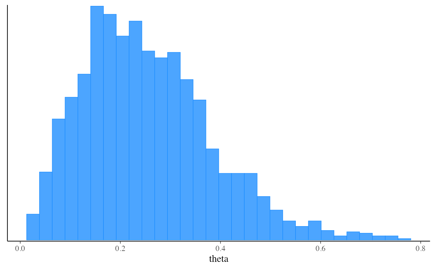
# Plot posterior using bayesplot (ggplot2)
mcmc_hist(fit_mcmc$draws("theta"))
#> `stat_bin()` using `bins = 30`. Pick better value with `binwidth`.
 # Run 'optimize' method to get a point estimate (default is Stan's LBFGS algorithm)
# and also demonstrate specifying data as a path to a file instead of a list
my_data_file <- file.path(cmdstan_path(), "examples/bernoulli/bernoulli.data.json")
fit_optim <- mod$optimize(data = my_data_file, seed = 123)
#> Initial log joint probability = -16.144
#> Iter log prob ||dx|| ||grad|| alpha alpha0 # evals Notes
#> 6 -5.00402 0.000246518 8.73164e-07 1 1 9
#> Optimization terminated normally:
#> Convergence detected: relative gradient magnitude is below tolerance
#> Finished in 0.1 seconds.
fit_optim$summary()
#> # A tibble: 2 × 2
#> variable estimate
#> <chr> <dbl>
#> 1 lp__ -5.00
#> 2 theta 0.2
# Run 'optimize' again with 'jacobian=TRUE' and then draw from Laplace approximation
# to the posterior
fit_optim <- mod$optimize(data = my_data_file, jacobian = TRUE)
#> Initial log joint probability = -6.80195
#> Iter log prob ||dx|| ||grad|| alpha alpha0 # evals Notes
#> 4 -6.74802 0.00029907 1.30133e-06 1 1 7
#> Optimization terminated normally:
#> Convergence detected: relative gradient magnitude is below tolerance
#> Finished in 0.1 seconds.
fit_laplace <- mod$laplace(data = my_data_file, mode = fit_optim, draws = 2000)
#> Calculating Hessian
#> Calculating inverse of Cholesky factor
#> Generating draws
#> iteration: 0
#> iteration: 100
#> iteration: 200
#> iteration: 300
#> iteration: 400
#> iteration: 500
#> iteration: 600
#> iteration: 700
#> iteration: 800
#> iteration: 900
#> iteration: 1000
#> iteration: 1100
#> iteration: 1200
#> iteration: 1300
#> iteration: 1400
#> iteration: 1500
#> iteration: 1600
#> iteration: 1700
#> iteration: 1800
#> iteration: 1900
#> Finished in 0.1 seconds.
fit_laplace$summary()
#> # A tibble: 3 × 7
#> variable mean median sd mad q5 q95
#> <chr> <dbl> <dbl> <dbl> <dbl> <dbl> <dbl>
#> 1 lp__ -7.22 -6.96 0.660 0.293 -8.56 -6.75
#> 2 lp_approx__ -0.479 -0.220 0.648 0.296 -1.85 -0.00230
#> 3 theta 0.271 0.251 0.122 0.119 0.101 0.501
# Run 'variational' method to use ADVI to approximate posterior
fit_vb <- mod$variational(data = stan_data, seed = 123)
#> ------------------------------------------------------------
#> EXPERIMENTAL ALGORITHM:
#> This procedure has not been thoroughly tested and may be unstable
#> or buggy. The interface is subject to change.
#> ------------------------------------------------------------
#> Gradient evaluation took 1e-05 seconds
#> 1000 transitions using 10 leapfrog steps per transition would take 0.1 seconds.
#> Adjust your expectations accordingly!
#> Begin eta adaptation.
#> Iteration: 1 / 250 [ 0%] (Adaptation)
#> Iteration: 50 / 250 [ 20%] (Adaptation)
#> Iteration: 100 / 250 [ 40%] (Adaptation)
#> Iteration: 150 / 250 [ 60%] (Adaptation)
#> Iteration: 200 / 250 [ 80%] (Adaptation)
#> Success! Found best value [eta = 1] earlier than expected.
#> Begin stochastic gradient ascent.
#> iter ELBO delta_ELBO_mean delta_ELBO_med notes
#> 100 -6.164 1.000 1.000
#> 200 -6.225 0.505 1.000
#> 300 -6.186 0.339 0.010 MEDIAN ELBO CONVERGED
#> Drawing a sample of size 1000 from the approximate posterior...
#> COMPLETED.
#> Finished in 0.1 seconds.
fit_vb$summary()
#> # A tibble: 3 × 7
#> variable mean median sd mad q5 q95
#> <chr> <dbl> <dbl> <dbl> <dbl> <dbl> <dbl>
#> 1 lp__ -7.14 -6.93 0.528 0.247 -8.21 -6.75
#> 2 lp_approx__ -0.520 -0.244 0.740 0.326 -1.90 -0.00227
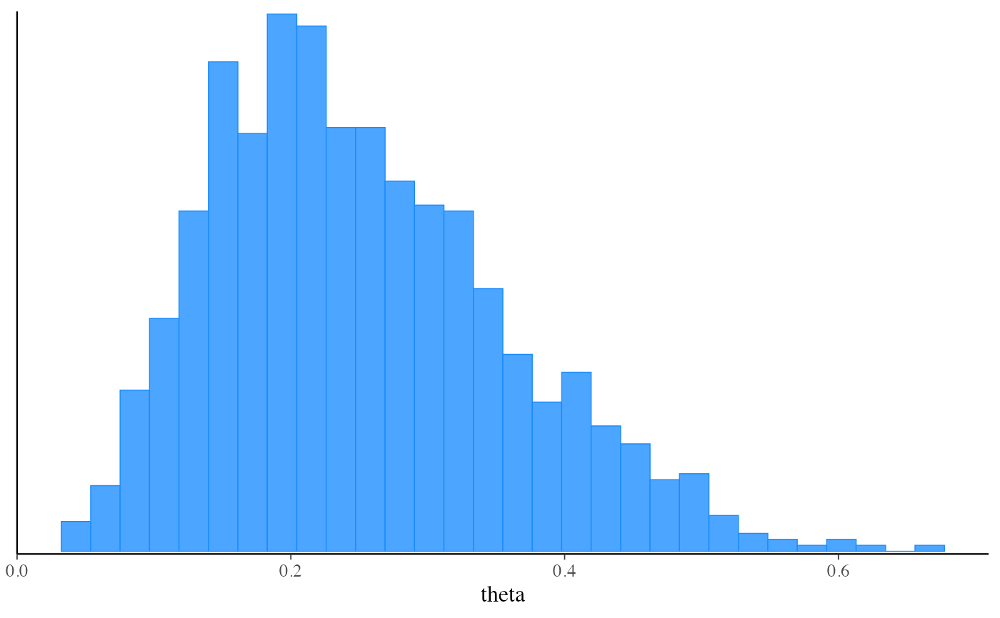
#> 3 theta 0.251 0.236 0.107 0.108 0.100 0.446
mcmc_hist(fit_vb$draws("theta"))
#> `stat_bin()` using `bins = 30`. Pick better value with `binwidth`.
# Run 'optimize' method to get a point estimate (default is Stan's LBFGS algorithm)
# and also demonstrate specifying data as a path to a file instead of a list
my_data_file <- file.path(cmdstan_path(), "examples/bernoulli/bernoulli.data.json")
fit_optim <- mod$optimize(data = my_data_file, seed = 123)
#> Initial log joint probability = -16.144
#> Iter log prob ||dx|| ||grad|| alpha alpha0 # evals Notes
#> 6 -5.00402 0.000246518 8.73164e-07 1 1 9
#> Optimization terminated normally:
#> Convergence detected: relative gradient magnitude is below tolerance
#> Finished in 0.1 seconds.
fit_optim$summary()
#> # A tibble: 2 × 2
#> variable estimate
#> <chr> <dbl>
#> 1 lp__ -5.00
#> 2 theta 0.2
# Run 'optimize' again with 'jacobian=TRUE' and then draw from Laplace approximation
# to the posterior
fit_optim <- mod$optimize(data = my_data_file, jacobian = TRUE)
#> Initial log joint probability = -6.80195
#> Iter log prob ||dx|| ||grad|| alpha alpha0 # evals Notes
#> 4 -6.74802 0.00029907 1.30133e-06 1 1 7
#> Optimization terminated normally:
#> Convergence detected: relative gradient magnitude is below tolerance
#> Finished in 0.1 seconds.
fit_laplace <- mod$laplace(data = my_data_file, mode = fit_optim, draws = 2000)
#> Calculating Hessian
#> Calculating inverse of Cholesky factor
#> Generating draws
#> iteration: 0
#> iteration: 100
#> iteration: 200
#> iteration: 300
#> iteration: 400
#> iteration: 500
#> iteration: 600
#> iteration: 700
#> iteration: 800
#> iteration: 900
#> iteration: 1000
#> iteration: 1100
#> iteration: 1200
#> iteration: 1300
#> iteration: 1400
#> iteration: 1500
#> iteration: 1600
#> iteration: 1700
#> iteration: 1800
#> iteration: 1900
#> Finished in 0.1 seconds.
fit_laplace$summary()
#> # A tibble: 3 × 7
#> variable mean median sd mad q5 q95
#> <chr> <dbl> <dbl> <dbl> <dbl> <dbl> <dbl>
#> 1 lp__ -7.22 -6.96 0.660 0.293 -8.56 -6.75
#> 2 lp_approx__ -0.479 -0.220 0.648 0.296 -1.85 -0.00230
#> 3 theta 0.271 0.251 0.122 0.119 0.101 0.501
# Run 'variational' method to use ADVI to approximate posterior
fit_vb <- mod$variational(data = stan_data, seed = 123)
#> ------------------------------------------------------------
#> EXPERIMENTAL ALGORITHM:
#> This procedure has not been thoroughly tested and may be unstable
#> or buggy. The interface is subject to change.
#> ------------------------------------------------------------
#> Gradient evaluation took 1e-05 seconds
#> 1000 transitions using 10 leapfrog steps per transition would take 0.1 seconds.
#> Adjust your expectations accordingly!
#> Begin eta adaptation.
#> Iteration: 1 / 250 [ 0%] (Adaptation)
#> Iteration: 50 / 250 [ 20%] (Adaptation)
#> Iteration: 100 / 250 [ 40%] (Adaptation)
#> Iteration: 150 / 250 [ 60%] (Adaptation)
#> Iteration: 200 / 250 [ 80%] (Adaptation)
#> Success! Found best value [eta = 1] earlier than expected.
#> Begin stochastic gradient ascent.
#> iter ELBO delta_ELBO_mean delta_ELBO_med notes
#> 100 -6.164 1.000 1.000
#> 200 -6.225 0.505 1.000
#> 300 -6.186 0.339 0.010 MEDIAN ELBO CONVERGED
#> Drawing a sample of size 1000 from the approximate posterior...
#> COMPLETED.
#> Finished in 0.1 seconds.
fit_vb$summary()
#> # A tibble: 3 × 7
#> variable mean median sd mad q5 q95
#> <chr> <dbl> <dbl> <dbl> <dbl> <dbl> <dbl>
#> 1 lp__ -7.14 -6.93 0.528 0.247 -8.21 -6.75
#> 2 lp_approx__ -0.520 -0.244 0.740 0.326 -1.90 -0.00227
#> 3 theta 0.251 0.236 0.107 0.108 0.100 0.446
mcmc_hist(fit_vb$draws("theta"))
#> `stat_bin()` using `bins = 30`. Pick better value with `binwidth`.
 # Run 'pathfinder' method, a new alternative to the variational method
fit_pf <- mod$pathfinder(data = stan_data, seed = 123)
#> Path [1] :Initial log joint density = -18.273334
#> Path [1] : Iter log prob ||dx|| ||grad|| alpha alpha0 # evals ELBO Best ELBO Notes
#> 5 -6.748e+00 7.082e-04 1.432e-05 1.000e+00 1.000e+00 126 -6.145e+00 -6.145e+00
#> Path [1] :Best Iter: [5] ELBO (-6.145070) evaluations: (126)
#> Path [2] :Initial log joint density = -19.192715
#> Path [2] : Iter log prob ||dx|| ||grad|| alpha alpha0 # evals ELBO Best ELBO Notes
#> 5 -6.748e+00 2.015e-04 2.228e-06 1.000e+00 1.000e+00 126 -6.223e+00 -6.223e+00
#> Path [2] :Best Iter: [2] ELBO (-6.170358) evaluations: (126)
#> Path [3] :Initial log joint density = -6.774820
#> Path [3] : Iter log prob ||dx|| ||grad|| alpha alpha0 # evals ELBO Best ELBO Notes
#> 4 -6.748e+00 1.137e-04 2.596e-07 1.000e+00 1.000e+00 101 -6.178e+00 -6.178e+00
#> Path [3] :Best Iter: [4] ELBO (-6.177909) evaluations: (101)
#> Path [4] :Initial log joint density = -7.949193
#> Path [4] : Iter log prob ||dx|| ||grad|| alpha alpha0 # evals ELBO Best ELBO Notes
#> 5 -6.748e+00 2.145e-04 1.301e-06 1.000e+00 1.000e+00 126 -6.197e+00 -6.197e+00
#> Path [4] :Best Iter: [5] ELBO (-6.197118) evaluations: (126)
#> Total log probability function evaluations:4379
#> Finished in 0.1 seconds.
fit_pf$summary()
#> # A tibble: 3 × 7
#> variable mean median sd mad q5 q95
#> <chr> <dbl> <dbl> <dbl> <dbl> <dbl> <dbl>
#> 1 lp_approx__ -1.07 -0.727 0.945 0.311 -2.91 -0.450
#> 2 lp__ -7.25 -6.97 0.753 0.308 -8.78 -6.75
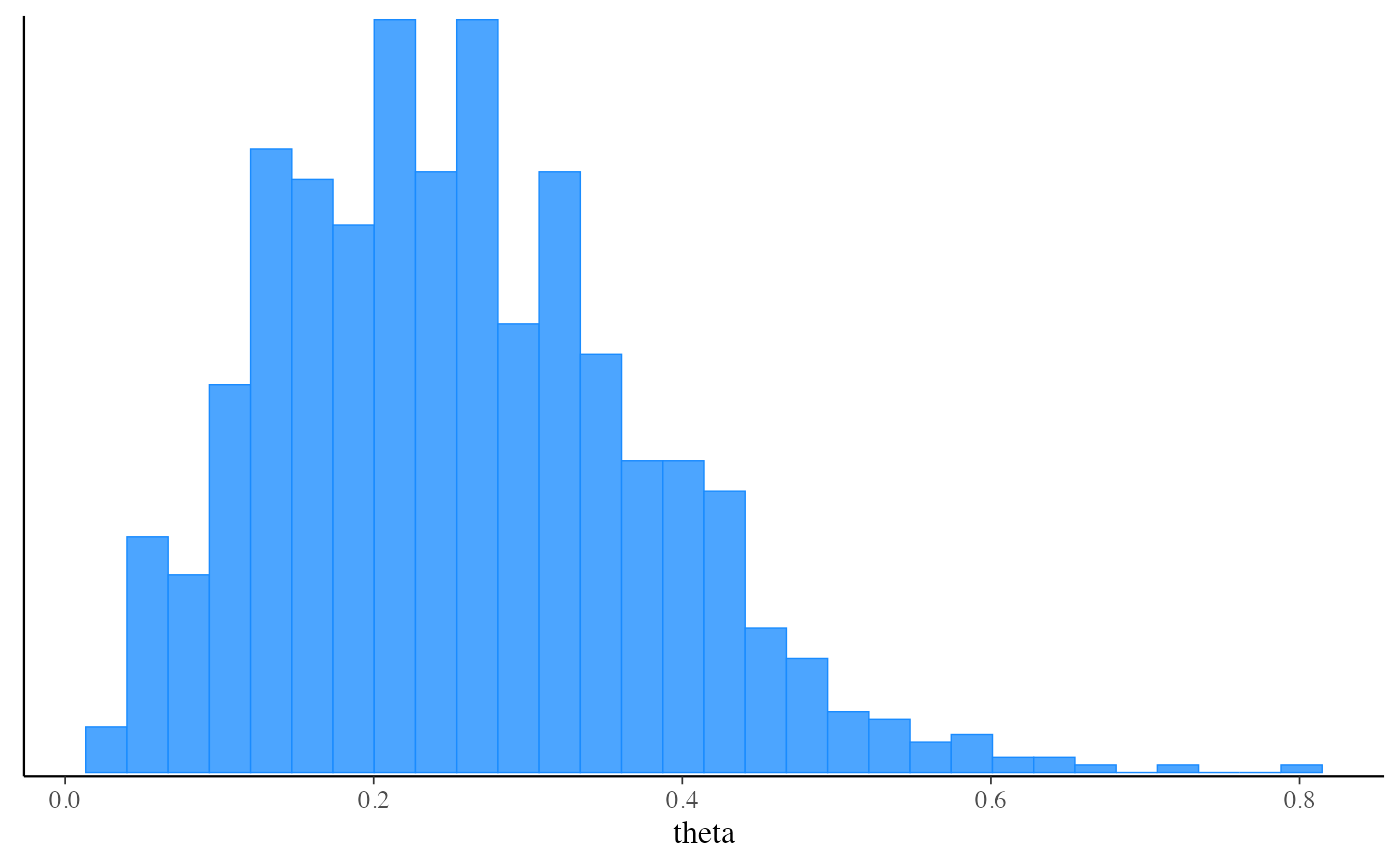
#> 3 theta 0.256 0.245 0.119 0.123 0.0824 0.462
mcmc_hist(fit_pf$draws("theta"))
#> `stat_bin()` using `bins = 30`. Pick better value with `binwidth`.
# Run 'pathfinder' method, a new alternative to the variational method
fit_pf <- mod$pathfinder(data = stan_data, seed = 123)
#> Path [1] :Initial log joint density = -18.273334
#> Path [1] : Iter log prob ||dx|| ||grad|| alpha alpha0 # evals ELBO Best ELBO Notes
#> 5 -6.748e+00 7.082e-04 1.432e-05 1.000e+00 1.000e+00 126 -6.145e+00 -6.145e+00
#> Path [1] :Best Iter: [5] ELBO (-6.145070) evaluations: (126)
#> Path [2] :Initial log joint density = -19.192715
#> Path [2] : Iter log prob ||dx|| ||grad|| alpha alpha0 # evals ELBO Best ELBO Notes
#> 5 -6.748e+00 2.015e-04 2.228e-06 1.000e+00 1.000e+00 126 -6.223e+00 -6.223e+00
#> Path [2] :Best Iter: [2] ELBO (-6.170358) evaluations: (126)
#> Path [3] :Initial log joint density = -6.774820
#> Path [3] : Iter log prob ||dx|| ||grad|| alpha alpha0 # evals ELBO Best ELBO Notes
#> 4 -6.748e+00 1.137e-04 2.596e-07 1.000e+00 1.000e+00 101 -6.178e+00 -6.178e+00
#> Path [3] :Best Iter: [4] ELBO (-6.177909) evaluations: (101)
#> Path [4] :Initial log joint density = -7.949193
#> Path [4] : Iter log prob ||dx|| ||grad|| alpha alpha0 # evals ELBO Best ELBO Notes
#> 5 -6.748e+00 2.145e-04 1.301e-06 1.000e+00 1.000e+00 126 -6.197e+00 -6.197e+00
#> Path [4] :Best Iter: [5] ELBO (-6.197118) evaluations: (126)
#> Total log probability function evaluations:4379
#> Finished in 0.1 seconds.
fit_pf$summary()
#> # A tibble: 3 × 7
#> variable mean median sd mad q5 q95
#> <chr> <dbl> <dbl> <dbl> <dbl> <dbl> <dbl>
#> 1 lp_approx__ -1.07 -0.727 0.945 0.311 -2.91 -0.450
#> 2 lp__ -7.25 -6.97 0.753 0.308 -8.78 -6.75
#> 3 theta 0.256 0.245 0.119 0.123 0.0824 0.462
mcmc_hist(fit_pf$draws("theta"))
#> `stat_bin()` using `bins = 30`. Pick better value with `binwidth`.
 # Run 'pathfinder' again with more paths, fewer draws per path,
# better covariance approximation, and fewer LBFGSs iterations
fit_pf <- mod$pathfinder(data = stan_data, num_paths=10, single_path_draws=40,
history_size=50, max_lbfgs_iters=100)
#> Warning: Number of PSIS draws is larger than the total number of draws returned by the single Pathfinders. This is likely unintentional and leads to re-sampling from the same draws.
#> Path [1] :Initial log joint density = -8.288264
#> Path [1] : Iter log prob ||dx|| ||grad|| alpha alpha0 # evals ELBO Best ELBO Notes
#> 5 -6.748e+00 2.788e-04 2.003e-06 1.000e+00 1.000e+00 126 -6.242e+00 -6.242e+00
#> Path [1] :Best Iter: [2] ELBO (-6.189407) evaluations: (126)
#> Path [2] :Initial log joint density = -7.122559
#> Path [2] : Iter log prob ||dx|| ||grad|| alpha alpha0 # evals ELBO Best ELBO Notes
#> 4 -6.748e+00 3.446e-03 7.646e-05 1.000e+00 1.000e+00 101 -6.267e+00 -6.267e+00
#> Path [2] :Best Iter: [2] ELBO (-6.217814) evaluations: (101)
#> Path [3] :Initial log joint density = -6.904847
#> Path [3] : Iter log prob ||dx|| ||grad|| alpha alpha0 # evals ELBO Best ELBO Notes
#> 4 -6.748e+00 1.217e-03 1.351e-05 1.000e+00 1.000e+00 101 -6.256e+00 -6.256e+00
#> Path [3] :Best Iter: [3] ELBO (-6.226443) evaluations: (101)
#> Path [4] :Initial log joint density = -15.810600
#> Path [4] : Iter log prob ||dx|| ||grad|| alpha alpha0 # evals ELBO Best ELBO Notes
#> 5 -6.748e+00 1.919e-03 5.787e-05 1.000e+00 1.000e+00 126 -6.202e+00 -6.202e+00
#> Path [4] :Best Iter: [4] ELBO (-6.144907) evaluations: (126)
#> Path [5] :Initial log joint density = -7.535814
#> Path [5] : Iter log prob ||dx|| ||grad|| alpha alpha0 # evals ELBO Best ELBO Notes
#> 5 -6.748e+00 1.206e-04 5.112e-07 1.000e+00 1.000e+00 126 -6.233e+00 -6.233e+00
#> Path [5] :Best Iter: [4] ELBO (-6.165244) evaluations: (126)
#> Path [6] :Initial log joint density = -12.317092
#> Path [6] : Iter log prob ||dx|| ||grad|| alpha alpha0 # evals ELBO Best ELBO Notes
#> 5 -6.748e+00 1.394e-03 2.744e-05 1.000e+00 1.000e+00 126 -6.247e+00 -6.247e+00
#> Path [6] :Best Iter: [3] ELBO (-6.207884) evaluations: (126)
#> Path [7] :Initial log joint density = -6.970206
#> Path [7] : Iter log prob ||dx|| ||grad|| alpha alpha0 # evals ELBO Best ELBO Notes
#> 4 -6.748e+00 3.919e-04 8.523e-05 9.151e-01 9.151e-01 101 -6.187e+00 -6.187e+00
#> Path [7] :Best Iter: [4] ELBO (-6.187348) evaluations: (101)
#> Path [8] :Initial log joint density = -6.960470
#> Path [8] : Iter log prob ||dx|| ||grad|| alpha alpha0 # evals ELBO Best ELBO Notes
#> 4 -6.748e+00 1.773e-03 2.529e-05 1.000e+00 1.000e+00 101 -6.148e+00 -6.148e+00
#> Path [8] :Best Iter: [4] ELBO (-6.147740) evaluations: (101)
#> Path [9] :Initial log joint density = -6.771981
#> Path [9] : Iter log prob ||dx|| ||grad|| alpha alpha0 # evals ELBO Best ELBO Notes
#> 3 -6.748e+00 2.126e-03 4.338e-07 9.709e-01 9.709e-01 76 -6.239e+00 -6.239e+00
#> Path [9] :Best Iter: [2] ELBO (-6.211440) evaluations: (76)
#> Path [10] :Initial log joint density = -7.099410
#> Path [10] : Iter log prob ||dx|| ||grad|| alpha alpha0 # evals ELBO Best ELBO Notes
#> 5 -6.748e+00 1.211e-04 7.078e-08 1.000e+00 1.000e+00 126 -6.227e+00 -6.227e+00
#> Path [10] :Best Iter: [2] ELBO (-6.196731) evaluations: (126)
#> Total log probability function evaluations:1260
#> Finished in 0.1 seconds.
# Specifying initial values as a function
fit_mcmc_w_init_fun <- mod$sample(
data = stan_data,
seed = 123,
chains = 2,
refresh = 0,
init = function() list(theta = runif(1))
)
#> Running MCMC with 2 sequential chains...
#>
#> Chain 1 finished in 0.0 seconds.
#> Chain 2 finished in 0.0 seconds.
#>
#> Both chains finished successfully.
#> Mean chain execution time: 0.0 seconds.
#> Total execution time: 0.3 seconds.
#>
fit_mcmc_w_init_fun_2 <- mod$sample(
data = stan_data,
seed = 123,
chains = 2,
refresh = 0,
init = function(chain_id) {
# silly but demonstrates optional use of chain_id
list(theta = 1 / (chain_id + 1))
}
)
#> Running MCMC with 2 sequential chains...
#>
#> Chain 1 finished in 0.0 seconds.
#> Chain 2 finished in 0.0 seconds.
#>
#> Both chains finished successfully.
#> Mean chain execution time: 0.0 seconds.
#> Total execution time: 0.3 seconds.
#>
fit_mcmc_w_init_fun_2$init()
#> [[1]]
#> [[1]]$theta
#> [1] 0.5
#>
#>
#> [[2]]
#> [[2]]$theta
#> [1] 0.3333333
#>
#>
# Specifying initial values as a list of lists
fit_mcmc_w_init_list <- mod$sample(
data = stan_data,
seed = 123,
chains = 2,
refresh = 0,
init = list(
list(theta = 0.75), # chain 1
list(theta = 0.25) # chain 2
)
)
#> Running MCMC with 2 sequential chains...
#>
#> Chain 1 finished in 0.0 seconds.
#> Chain 2 finished in 0.0 seconds.
#>
#> Both chains finished successfully.
#> Mean chain execution time: 0.0 seconds.
#> Total execution time: 0.3 seconds.
#>
fit_optim_w_init_list <- mod$optimize(
data = stan_data,
seed = 123,
init = list(
list(theta = 0.75)
)
)
#> Initial log joint probability = -11.6657
#> Iter log prob ||dx|| ||grad|| alpha alpha0 # evals Notes
#> 6 -5.00402 0.000237915 9.55309e-07 1 1 9
#> Optimization terminated normally:
#> Convergence detected: relative gradient magnitude is below tolerance
#> Finished in 0.1 seconds.
fit_optim_w_init_list$init()
#> [[1]]
#> [[1]]$theta
#> [1] 0.75
#>
#>
# }
# Run 'pathfinder' again with more paths, fewer draws per path,
# better covariance approximation, and fewer LBFGSs iterations
fit_pf <- mod$pathfinder(data = stan_data, num_paths=10, single_path_draws=40,
history_size=50, max_lbfgs_iters=100)
#> Warning: Number of PSIS draws is larger than the total number of draws returned by the single Pathfinders. This is likely unintentional and leads to re-sampling from the same draws.
#> Path [1] :Initial log joint density = -8.288264
#> Path [1] : Iter log prob ||dx|| ||grad|| alpha alpha0 # evals ELBO Best ELBO Notes
#> 5 -6.748e+00 2.788e-04 2.003e-06 1.000e+00 1.000e+00 126 -6.242e+00 -6.242e+00
#> Path [1] :Best Iter: [2] ELBO (-6.189407) evaluations: (126)
#> Path [2] :Initial log joint density = -7.122559
#> Path [2] : Iter log prob ||dx|| ||grad|| alpha alpha0 # evals ELBO Best ELBO Notes
#> 4 -6.748e+00 3.446e-03 7.646e-05 1.000e+00 1.000e+00 101 -6.267e+00 -6.267e+00
#> Path [2] :Best Iter: [2] ELBO (-6.217814) evaluations: (101)
#> Path [3] :Initial log joint density = -6.904847
#> Path [3] : Iter log prob ||dx|| ||grad|| alpha alpha0 # evals ELBO Best ELBO Notes
#> 4 -6.748e+00 1.217e-03 1.351e-05 1.000e+00 1.000e+00 101 -6.256e+00 -6.256e+00
#> Path [3] :Best Iter: [3] ELBO (-6.226443) evaluations: (101)
#> Path [4] :Initial log joint density = -15.810600
#> Path [4] : Iter log prob ||dx|| ||grad|| alpha alpha0 # evals ELBO Best ELBO Notes
#> 5 -6.748e+00 1.919e-03 5.787e-05 1.000e+00 1.000e+00 126 -6.202e+00 -6.202e+00
#> Path [4] :Best Iter: [4] ELBO (-6.144907) evaluations: (126)
#> Path [5] :Initial log joint density = -7.535814
#> Path [5] : Iter log prob ||dx|| ||grad|| alpha alpha0 # evals ELBO Best ELBO Notes
#> 5 -6.748e+00 1.206e-04 5.112e-07 1.000e+00 1.000e+00 126 -6.233e+00 -6.233e+00
#> Path [5] :Best Iter: [4] ELBO (-6.165244) evaluations: (126)
#> Path [6] :Initial log joint density = -12.317092
#> Path [6] : Iter log prob ||dx|| ||grad|| alpha alpha0 # evals ELBO Best ELBO Notes
#> 5 -6.748e+00 1.394e-03 2.744e-05 1.000e+00 1.000e+00 126 -6.247e+00 -6.247e+00
#> Path [6] :Best Iter: [3] ELBO (-6.207884) evaluations: (126)
#> Path [7] :Initial log joint density = -6.970206
#> Path [7] : Iter log prob ||dx|| ||grad|| alpha alpha0 # evals ELBO Best ELBO Notes
#> 4 -6.748e+00 3.919e-04 8.523e-05 9.151e-01 9.151e-01 101 -6.187e+00 -6.187e+00
#> Path [7] :Best Iter: [4] ELBO (-6.187348) evaluations: (101)
#> Path [8] :Initial log joint density = -6.960470
#> Path [8] : Iter log prob ||dx|| ||grad|| alpha alpha0 # evals ELBO Best ELBO Notes
#> 4 -6.748e+00 1.773e-03 2.529e-05 1.000e+00 1.000e+00 101 -6.148e+00 -6.148e+00
#> Path [8] :Best Iter: [4] ELBO (-6.147740) evaluations: (101)
#> Path [9] :Initial log joint density = -6.771981
#> Path [9] : Iter log prob ||dx|| ||grad|| alpha alpha0 # evals ELBO Best ELBO Notes
#> 3 -6.748e+00 2.126e-03 4.338e-07 9.709e-01 9.709e-01 76 -6.239e+00 -6.239e+00
#> Path [9] :Best Iter: [2] ELBO (-6.211440) evaluations: (76)
#> Path [10] :Initial log joint density = -7.099410
#> Path [10] : Iter log prob ||dx|| ||grad|| alpha alpha0 # evals ELBO Best ELBO Notes
#> 5 -6.748e+00 1.211e-04 7.078e-08 1.000e+00 1.000e+00 126 -6.227e+00 -6.227e+00
#> Path [10] :Best Iter: [2] ELBO (-6.196731) evaluations: (126)
#> Total log probability function evaluations:1260
#> Finished in 0.1 seconds.
# Specifying initial values as a function
fit_mcmc_w_init_fun <- mod$sample(
data = stan_data,
seed = 123,
chains = 2,
refresh = 0,
init = function() list(theta = runif(1))
)
#> Running MCMC with 2 sequential chains...
#>
#> Chain 1 finished in 0.0 seconds.
#> Chain 2 finished in 0.0 seconds.
#>
#> Both chains finished successfully.
#> Mean chain execution time: 0.0 seconds.
#> Total execution time: 0.3 seconds.
#>
fit_mcmc_w_init_fun_2 <- mod$sample(
data = stan_data,
seed = 123,
chains = 2,
refresh = 0,
init = function(chain_id) {
# silly but demonstrates optional use of chain_id
list(theta = 1 / (chain_id + 1))
}
)
#> Running MCMC with 2 sequential chains...
#>
#> Chain 1 finished in 0.0 seconds.
#> Chain 2 finished in 0.0 seconds.
#>
#> Both chains finished successfully.
#> Mean chain execution time: 0.0 seconds.
#> Total execution time: 0.3 seconds.
#>
fit_mcmc_w_init_fun_2$init()
#> [[1]]
#> [[1]]$theta
#> [1] 0.5
#>
#>
#> [[2]]
#> [[2]]$theta
#> [1] 0.3333333
#>
#>
# Specifying initial values as a list of lists
fit_mcmc_w_init_list <- mod$sample(
data = stan_data,
seed = 123,
chains = 2,
refresh = 0,
init = list(
list(theta = 0.75), # chain 1
list(theta = 0.25) # chain 2
)
)
#> Running MCMC with 2 sequential chains...
#>
#> Chain 1 finished in 0.0 seconds.
#> Chain 2 finished in 0.0 seconds.
#>
#> Both chains finished successfully.
#> Mean chain execution time: 0.0 seconds.
#> Total execution time: 0.3 seconds.
#>
fit_optim_w_init_list <- mod$optimize(
data = stan_data,
seed = 123,
init = list(
list(theta = 0.75)
)
)
#> Initial log joint probability = -11.6657
#> Iter log prob ||dx|| ||grad|| alpha alpha0 # evals Notes
#> 6 -5.00402 0.000237915 9.55309e-07 1 1 9
#> Optimization terminated normally:
#> Convergence detected: relative gradient magnitude is below tolerance
#> Finished in 0.1 seconds.
fit_optim_w_init_list$init()
#> [[1]]
#> [[1]]$theta
#> [1] 0.75
#>
#>
# }