Plots for stanfit objects

The default plot shows posterior uncertainty intervals and point estimates for parameters and generated quantities. The plot method can also be used to call the other rstan plotting functions via the plotfun argument (see Examples).

Usage

# S4 method for class 'stanfit,missing'
plot(x, ..., plotfun)

Arguments

x: An instance of class stanfit.
plotfun: A character string naming the plotting function to apply to the stanfit object. If plotfun is missing, the default is to call stan_plot, which generates a plot of credible intervals and point estimates. See rstan-plotting-functions for the names and descriptions of the other plotting functions. plotfun can be either the full name of the plotting function (e.g. "stan_hist") or can be abbreviated to the part of the name following the underscore (e.g. "hist").
...: Optional arguments to plotfun.

Value

A ggplot object that can be further customized using the ggplot2 package.

Note

Because the rstan plotting functions use ggplot2 (and thus the resulting plots behave like ggplot objects), when calling a plotting function within a loop or when assigning a plot to a name (e.g., graph <- plot(fit, plotfun = "rhat")), if you also want the side effect of the plot being displayed you must explicity print it (e.g., (graph <- plot(fit, plotfun = "rhat")), print(graph <- plot(fit, plotfun = "rhat"))).

Examples

# \dontrun{
library(rstan)
fit <- stan_demo("eight_schools")
#> 
#> > J <- 8
#> 
#> > y <- c(28, 8, -3, 7, -1, 1, 18, 12)
#> 
#> > sigma <- c(15, 10, 16, 11, 9, 11, 10, 18)
#> 
#> > tau <- 25
#> 
#> SAMPLING FOR MODEL 'eight_schools' NOW (CHAIN 1).
#> Chain 1: 
#> Chain 1: Gradient evaluation took 5e-06 seconds
#> Chain 1: 1000 transitions using 10 leapfrog steps per transition would take 0.05 seconds.
#> Chain 1: Adjust your expectations accordingly!
#> Chain 1: 
#> Chain 1: 
#> Chain 1: Iteration:    1 / 2000 [  0%]  (Warmup)
#> Chain 1: Iteration:  200 / 2000 [ 10%]  (Warmup)
#> Chain 1: Iteration:  400 / 2000 [ 20%]  (Warmup)
#> Chain 1: Iteration:  600 / 2000 [ 30%]  (Warmup)
#> Chain 1: Iteration:  800 / 2000 [ 40%]  (Warmup)
#> Chain 1: Iteration: 1000 / 2000 [ 50%]  (Warmup)
#> Chain 1: Iteration: 1001 / 2000 [ 50%]  (Sampling)
#> Chain 1: Iteration: 1200 / 2000 [ 60%]  (Sampling)
#> Chain 1: Iteration: 1400 / 2000 [ 70%]  (Sampling)
#> Chain 1: Iteration: 1600 / 2000 [ 80%]  (Sampling)
#> Chain 1: Iteration: 1800 / 2000 [ 90%]  (Sampling)
#> Chain 1: Iteration: 2000 / 2000 [100%]  (Sampling)
#> Chain 1: 
#> Chain 1:  Elapsed Time: 0.035 seconds (Warm-up)
#> Chain 1:                0.019 seconds (Sampling)
#> Chain 1:                0.054 seconds (Total)
#> Chain 1: 
#> 
#> SAMPLING FOR MODEL 'eight_schools' NOW (CHAIN 2).
#> Chain 2: 
#> Chain 2: Gradient evaluation took 2e-06 seconds
#> Chain 2: 1000 transitions using 10 leapfrog steps per transition would take 0.02 seconds.
#> Chain 2: Adjust your expectations accordingly!
#> Chain 2: 
#> Chain 2: 
#> Chain 2: Iteration:    1 / 2000 [  0%]  (Warmup)
#> Chain 2: Iteration:  200 / 2000 [ 10%]  (Warmup)
#> Chain 2: Iteration:  400 / 2000 [ 20%]  (Warmup)
#> Chain 2: Iteration:  600 / 2000 [ 30%]  (Warmup)
#> Chain 2: Iteration:  800 / 2000 [ 40%]  (Warmup)
#> Chain 2: Iteration: 1000 / 2000 [ 50%]  (Warmup)
#> Chain 2: Iteration: 1001 / 2000 [ 50%]  (Sampling)
#> Chain 2: Iteration: 1200 / 2000 [ 60%]  (Sampling)
#> Chain 2: Iteration: 1400 / 2000 [ 70%]  (Sampling)
#> Chain 2: Iteration: 1600 / 2000 [ 80%]  (Sampling)
#> Chain 2: Iteration: 1800 / 2000 [ 90%]  (Sampling)
#> Chain 2: Iteration: 2000 / 2000 [100%]  (Sampling)
#> Chain 2: 
#> Chain 2:  Elapsed Time: 0.041 seconds (Warm-up)
#> Chain 2:                0.019 seconds (Sampling)
#> Chain 2:                0.06 seconds (Total)
#> Chain 2: 
#> 
#> SAMPLING FOR MODEL 'eight_schools' NOW (CHAIN 3).
#> Chain 3: 
#> Chain 3: Gradient evaluation took 2e-06 seconds
#> Chain 3: 1000 transitions using 10 leapfrog steps per transition would take 0.02 seconds.
#> Chain 3: Adjust your expectations accordingly!
#> Chain 3: 
#> Chain 3: 
#> Chain 3: Iteration:    1 / 2000 [  0%]  (Warmup)
#> Chain 3: Iteration:  200 / 2000 [ 10%]  (Warmup)
#> Chain 3: Iteration:  400 / 2000 [ 20%]  (Warmup)
#> Chain 3: Iteration:  600 / 2000 [ 30%]  (Warmup)
#> Chain 3: Iteration:  800 / 2000 [ 40%]  (Warmup)
#> Chain 3: Iteration: 1000 / 2000 [ 50%]  (Warmup)
#> Chain 3: Iteration: 1001 / 2000 [ 50%]  (Sampling)
#> Chain 3: Iteration: 1200 / 2000 [ 60%]  (Sampling)
#> Chain 3: Iteration: 1400 / 2000 [ 70%]  (Sampling)
#> Chain 3: Iteration: 1600 / 2000 [ 80%]  (Sampling)
#> Chain 3: Iteration: 1800 / 2000 [ 90%]  (Sampling)
#> Chain 3: Iteration: 2000 / 2000 [100%]  (Sampling)
#> Chain 3: 
#> Chain 3:  Elapsed Time: 0.033 seconds (Warm-up)
#> Chain 3:                0.017 seconds (Sampling)
#> Chain 3:                0.05 seconds (Total)
#> Chain 3: 
#> 
#> SAMPLING FOR MODEL 'eight_schools' NOW (CHAIN 4).
#> Chain 4: 
#> Chain 4: Gradient evaluation took 2e-06 seconds
#> Chain 4: 1000 transitions using 10 leapfrog steps per transition would take 0.02 seconds.
#> Chain 4: Adjust your expectations accordingly!
#> Chain 4: 
#> Chain 4: 
#> Chain 4: Iteration:    1 / 2000 [  0%]  (Warmup)
#> Chain 4: Iteration:  200 / 2000 [ 10%]  (Warmup)
#> Chain 4: Iteration:  400 / 2000 [ 20%]  (Warmup)
#> Chain 4: Iteration:  600 / 2000 [ 30%]  (Warmup)
#> Chain 4: Iteration:  800 / 2000 [ 40%]  (Warmup)
#> Chain 4: Iteration: 1000 / 2000 [ 50%]  (Warmup)
#> Chain 4: Iteration: 1001 / 2000 [ 50%]  (Sampling)
#> Chain 4: Iteration: 1200 / 2000 [ 60%]  (Sampling)
#> Chain 4: Iteration: 1400 / 2000 [ 70%]  (Sampling)
#> Chain 4: Iteration: 1600 / 2000 [ 80%]  (Sampling)
#> Chain 4: Iteration: 1800 / 2000 [ 90%]  (Sampling)
#> Chain 4: Iteration: 2000 / 2000 [100%]  (Sampling)
#> Chain 4: 
#> Chain 4:  Elapsed Time: 0.039 seconds (Warm-up)
#> Chain 4:                0.029 seconds (Sampling)
#> Chain 4:                0.068 seconds (Total)
#> Chain 4: 
#> Warning: There were 125 divergent transitions after warmup. See
#> https://mc-stan.org/misc/warnings.html#divergent-transitions-after-warmup
#> to find out why this is a problem and how to eliminate them.
#> Warning: Examine the pairs() plot to diagnose sampling problems
#> Warning: Bulk Effective Samples Size (ESS) is too low, indicating posterior means and medians may be unreliable.
#> Running the chains for more iterations may help. See
#> https://mc-stan.org/misc/warnings.html#bulk-ess
#> Warning: Tail Effective Samples Size (ESS) is too low, indicating posterior variances and tail quantiles may be unreliable.
#> Running the chains for more iterations may help. See
#> https://mc-stan.org/misc/warnings.html#tail-ess
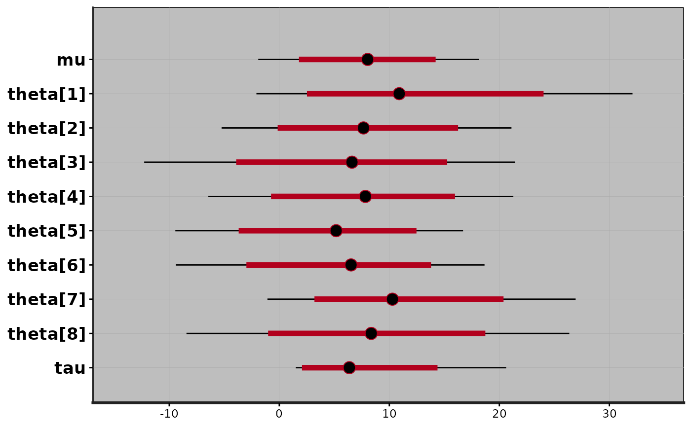
plot(fit)
#> ci_level: 0.8 (80% intervals)
#> outer_level: 0.95 (95% intervals)

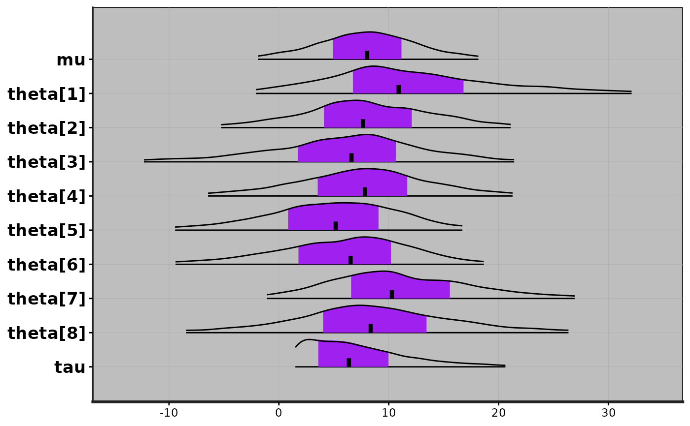
plot(fit, show_density = TRUE, ci_level = 0.5, fill_color = "purple")
#> ci_level: 0.5 (50% intervals)
#> outer_level: 0.95 (95% intervals)

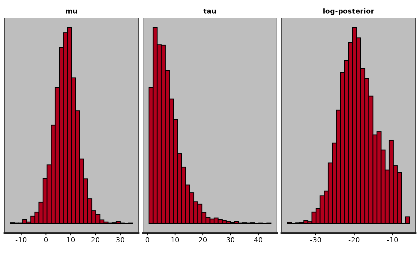
plot(fit, plotfun = "hist", pars = "theta", include = FALSE)
#> `stat_bin()` using `bins = 30`. Pick better value `binwidth`.

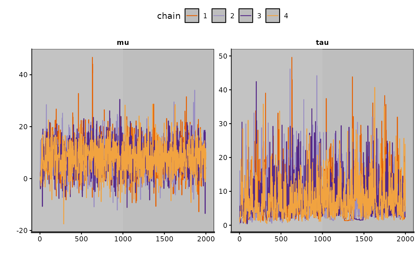
plot(fit, plotfun = "trace", pars = c("mu", "tau"), inc_warmup = TRUE)

plot(fit, plotfun = "rhat") + ggtitle("Example of adding title to plot")
#> Error in ggtitle("Example of adding title to plot"): could not find function "ggtitle"
# }

Usage

Arguments

Value

Note

See also

Examples