Loop over draws

Executes an expression once for every draw in a draws object. Used primarily for its side effects and returns the input x invisibly.

Usage

for_each_draw(x, expr)

Arguments

x

(draws) A draws object or another R object for which the method is defined.

expr

(expression) A bare expression that can contain references to variables in x by name. This expression will be executed once per draw of x, where references to variables in x resolve to the value of that variable in that draw. The expression supports quasiquotation.

Value

As for_each_draw() is used primarily for its side effects (the expression executed for each draw of x), it returns the input x invisibly.

Details

If x is not in the draws_rvars format, it is first converted to that format. This allows the variables in x to include their dimensions (i.e, to act as R vectors and arrays) when being referred to in expr.

Within expr, use .draw to refer to the draw index, which will be a value between 1 and ndraws(x). expr is executed in the calling environment of for_each_draw(), so it can use variables in that environment (however, due to the use of data masking, to modify variables in that environment, one must use <<-.)

Examples

eight_schools <- as_draws_rvars(example_draws())


# 1. A simple example --- looping over draws and printing each draw
# NOTE: You probably don't want to do this in practice! This example is
# just intended to show what for_each_draw() is doing. If you just want to
# print the draws of an rvar, it is probably better to use draws_of()
for_each_draw(eight_schools, {
  print(mu)
})
#> [1] 2.005831
#> [1] 1.458316
#> [1] 5.814947
#> [1] 6.849586
#> [1] 1.805168
#> [1] 3.841243
#> [1] 5.474273
#> [1] 1.203062
#> [1] 0.1463805
#> [1] 7.17291
#> [1] 0.9910314
#> [1] -1.550489
#> [1] 0.5842059
#> [1] 5.447506
#> [1] 6.180503
#> [1] 8.188255
#> [1] 7.384924
#> [1] 5.065307
#> [1] 6.59501
#> [1] -5.56139
#> [1] 10.34668
#> [1] 8.732913
#> [1] 8.560648
#> [1] 9.382581
#> [1] 1.368601
#> [1] 6.328316
#> [1] 7.920994
#> [1] 5.504498
#> [1] 7.154337
#> [1] 7.154337
#> [1] 4.498041
#> [1] 3.972859
#> [1] 1.246672
#> [1] 6.715447
#> [1] 2.593476
#> [1] 4.150923
#> [1] 5.576988
#> [1] 6.479588
#> [1] 6.714915
#> [1] 3.092834
#> [1] 4.667634
#> [1] 0.3257462
#> [1] 7.78165
#> [1] 2.771024
#> [1] -2.159893
#> [1] 3.623976
#> [1] 4.177537
#> [1] 5.189134
#> [1] 3.700737
#> [1] 8.054184
#> [1] 2.589031
#> [1] 2.482616
#> [1] 0.9075757
#> [1] 0.27648
#> [1] 8.077656
#> [1] 2.332971
#> [1] 4.332468
#> [1] 1.729912
#> [1] 1.419623
#> [1] 6.577866
#> [1] 11.08855
#> [1] -2.140353
#> [1] -1.800176
#> [1] 12.28125
#> [1] -2.614854
#> [1] 12.24904
#> [1] 0.8886184
#> [1] 0.9028057
#> [1] 1.677317
#> [1] 7.796531
#> [1] 9.592966
#> [1] 5.919053
#> [1] 2.746375
#> [1] 6.479243
#> [1] 2.768363
#> [1] 7.426639
#> [1] 2.667748
#> [1] 5.528707
#> [1] 11.79623
#> [1] -0.6559906
#> [1] -0.2416307
#> [1] 5.276274
#> [1] -0.1637204
#> [1] 1.761676
#> [1] -0.8038231
#> [1] 5.327505
#> [1] 6.328764
#> [1] 2.452526
#> [1] 3.733484
#> [1] 2.7919
#> [1] 6.123445
#> [1] 3.651789
#> [1] 5.425331
#> [1] 4.815524
#> [1] 3.507938
#> [1] 6.775166
#> [1] 1.856798
#> [1] 6.172828
#> [1] 1.548535
#> [1] 7.516744
#> [1] 2.990381
#> [1] 8.172526
#> [1] -1.15365
#> [1] 10.93486
#> [1] 9.820921
#> [1] -10.90481
#> [1] -9.260446
#> [1] 1.791052
#> [1] 5.350254
#> [1] 0.8686961
#> [1] 9.831286
#> [1] 7.178421
#> [1] 7.303903
#> [1] 0.1740227
#> [1] 8.024494
#> [1] 13.71125
#> [1] -2.654716
#> [1] 9.164643
#> [1] 7.337641
#> [1] -0.4282678
#> [1] 4.826956
#> [1] -0.421578
#> [1] 0.8573548
#> [1] 0.2247874
#> [1] 8.471193
#> [1] 9.4772
#> [1] 0.1802919
#> [1] 3.526179
#> [1] 6.635041
#> [1] 4.873137
#> [1] 5.749479
#> [1] -0.2319217
#> [1] 9.551073
#> [1] 1.256314
#> [1] 4.600533
#> [1] 2.622144
#> [1] 7.089645
#> [1] 3.271309
#> [1] 10.1848
#> [1] -2.222072
#> [1] 5.777605
#> [1] 3.345942
#> [1] 4.580048
#> [1] 6.25215
#> [1] 3.036535
#> [1] 6.377873
#> [1] -0.8467208
#> [1] 10.17687
#> [1] 2.262151
#> [1] 1.947261
#> [1] 8.905462
#> [1] 6.451443
#> [1] 4.76286
#> [1] -2.212966
#> [1] 8.292972
#> [1] 6.414798
#> [1] 6.069405
#> [1] 3.430352
#> [1] 4.860967
#> [1] 6.715199
#> [1] 7.275805
#> [1] 6.428511
#> [1] 3.242366
#> [1] 9.293644
#> [1] -0.6929381
#> [1] 8.700848
#> [1] 3.719785
#> [1] 5.747341
#> [1] 6.778653
#> [1] 8.779596
#> [1] 0.3407823
#> [1] 9.734953
#> [1] -1.61732
#> [1] 10.80919
#> [1] 2.96836
#> [1] 7.013745
#> [1] 3.666725
#> [1] 1.410787
#> [1] 6.585366
#> [1] 3.456987
#> [1] 3.942221
#> [1] 5.830744
#> [1] 7.50853
#> [1] -0.9847083
#> [1] 7.009851
#> [1] 1.248523
#> [1] 1.869871
#> [1] 5.82212
#> [1] 3.379486
#> [1] 5.587379
#> [1] 5.892139
#> [1] 10.19627
#> [1] 3.957886
#> [1] 2.666729
#> [1] 7.741973
#> [1] 0.7657729
#> [1] 8.243569
#> [1] 1.519901
#> [1] 8.575984
#> [1] -1.241991
#> [1] 1.794368
#> [1] 5.986371
#> [1] 2.557202
#> [1] 2.794425
#> [1] -0.02958928
#> [1] 1.063617
#> [1] 3.673857
#> [1] 3.505838
#> [1] 8.853159
#> [1] 8.853159
#> [1] 1.896446
#> [1] 4.269309
#> [1] 0.3929587
#> [1] -0.3855215
#> [1] 0.4399129
#> [1] 6.107962
#> [1] 6.136167
#> [1] 0.9391723
#> [1] -0.3633222
#> [1] 4.018959
#> [1] 5.360394
#> [1] 0.4944048
#> [1] 2.182324
#> [1] -0.450423
#> [1] 2.371517
#> [1] 1.998246
#> [1] 3.006006
#> [1] 2.614495
#> [1] 4.054033
#> [1] 4.727055
#> [1] 2.077013
#> [1] 1.7171
#> [1] 5.676568
#> [1] 7.359798
#> [1] 3.347586
#> [1] 3.465405
#> [1] 7.734784
#> [1] 1.075762
#> [1] 0.8731733
#> [1] 8.382703
#> [1] 9.133231
#> [1] 7.911396
#> [1] 3.647458
#> [1] 4.021722
#> [1] 5.590273
#> [1] 3.771822
#> [1] 6.767269
#> [1] 6.73121
#> [1] -2.035578
#> [1] -0.6331069
#> [1] -2.500302
#> [1] 8.864541
#> [1] 9.813685
#> [1] 4.852993
#> [1] -0.1317092
#> [1] 5.444751
#> [1] 6.496114
#> [1] 2.082844
#> [1] 3.426155
#> [1] 3.866463
#> [1] 1.897673
#> [1] 6.787045
#> [1] 3.676815
#> [1] 2.801344
#> [1] 1.558138
#> [1] 5.079696
#> [1] 5.331685
#> [1] 4.058808
#> [1] 6.433192
#> [1] 6.149452
#> [1] 6.754594
#> [1] 5.755464
#> [1] 4.770074
#> [1] 4.443709
#> [1] 6.27212
#> [1] 3.151525
#> [1] 4.954608
#> [1] 5.294373
#> [1] 3.509907
#> [1] -0.5068128
#> [1] -0.5068128
#> [1] -0.5068128
#> [1] -0.5068128
#> [1] 1.006574
#> [1] 3.142413
#> [1] 6.640588
#> [1] 4.788217
#> [1] 2.894039
#> [1] 9.07924
#> [1] 0.2812174
#> [1] 6.380328
#> [1] 7.482811
#> [1] 8.413412
#> [1] 6.317088
#> [1] 1.339948
#> [1] 7.774194
#> [1] 3.926885
#> [1] 0.08176881
#> [1] 3.174703
#> [1] 3.575558
#> [1] 6.458979
#> [1] 9.145118
#> [1] 0.2030693
#> [1] 3.692529
#> [1] 5.480271
#> [1] 2.379514
#> [1] 11.82462
#> [1] 4.90456
#> [1] 0.8796356
#> [1] 3.813747
#> [1] 3.432436
#> [1] -4.296498
#> [1] -4.06038
#> [1] 7.379277
#> [1] 2.212441
#> [1] 6.090105
#> [1] 8.645111
#> [1] 10.29126
#> [1] 2.295806
#> [1] 8.158265
#> [1] 6.594462
#> [1] 4.773796
#> [1] -1.60865
#> [1] 8.442649
#> [1] 1.968831
#> [1] 5.527651
#> [1] 6.100609
#> [1] 5.13686
#> [1] 6.267986
#> [1] 6.21822
#> [1] 2.246441
#> [1] 1.015631
#> [1] 4.376825
#> [1] -0.2470492
#> [1] 6.855368
#> [1] 0.7892017
#> [1] 7.310153
#> [1] 0.5838083
#> [1] 3.452831
#> [1] 6.157008
#> [1] 6.945902
#> [1] 7.793461
#> [1] 5.713618
#> [1] 1.094745
#> [1] 4.14184
#> [1] 4.656109
#> [1] 4.835303
#> [1] 2.360251
#> [1] 5.1895
#> [1] 6.964457
#> [1] 0.7819602
#> [1] 4.921984
#> [1] 4.125013
#> [1] 4.381954
#> [1] 0.4576623
#> [1] 3.089239
#> [1] 5.613297
#> [1] 5.800871
#> [1] 2.689139
#> [1] 4.23484
#> [1] -0.1137887
#> [1] 6.758072
#> [1] 5.357305
#> [1] 3.36597
#> [1] 3.614427
#> [1] 3.357607
#> [1] 3.627169
#> [1] 0.8046778
#> [1] 7.199353
#> [1] -0.3494357
#> [1] 1.544988
#> [1] 8.613144
#> [1] 0.5170308
#> [1] 8.365525
#> [1] 0.9939937
#> [1] 2.543458
#> [1] 7.218512
#> [1] 5.124879
#> [1] 2.415208
#> [1] 3.815243
#> [1] 5.156247
#> [1] 3.742969
#> [1] 0.4044733
#> [1] 8.137713
#> [1] 8.008371
#> [1] 6.180301
#> [1] 5.815311
#> [1] 3.155752
#> [1] 3.224573
#> [1] 5.446791
#> [1] 1.068988
#> [1] 6.694287
#> [1] 5.169541
#> [1] 0.9799776
#> [1] 5.687312
#> [1] 3.280556
#> [1] 5.039586
#> [1] 2.726364
#> [1] 0.4754905
#> [1] 7.047233


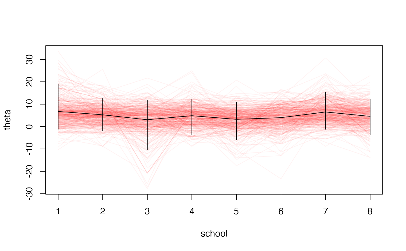
# 2. A more complex example --- building a parallel coordinates plot
# First, construct the plot bounds
plot(1, type = "n",
  xlim = c(1, length(eight_schools$theta)),
  ylim = range(range(eight_schools$theta)),
  xlab = "school", ylab = "theta"
)

# Then, use for_each_draw() to make a parallel coordinates plot of all draws
# of eight_schools$theta. Use resample_draws(eight_schools, n = ...)
# in place of eight_schools if a smaller sample is desired for the plot.
for_each_draw(eight_schools, {
  lines(seq_along(theta), theta, col = rgb(1, 0, 0, 0.05))
})

# Finally, add means and 90% intervals
lines(seq_along(eight_schools$theta), mean(eight_schools$theta))
with(summarise_draws(eight_schools$theta),
  segments(seq_along(eight_schools$theta), y0 = q5, y1 = q95)
)