20.1 Collinearity of Predictors in Regressions
This section discusses problems related to the classical notion of identifiability, which lead to ridges in the posterior density and wreak havoc with both sampling and inference.
Examples of Collinearity
Redundant Intercepts
The first example of collinearity is an artificial example involving redundant intercept parameters.33
Suppose there are observations \(y_n\) for \(n \in \{1,\dotsc,N\}\), two intercept parameters \(\lambda_1\) and \(\lambda_2\), a scale parameter \(\sigma > 0\), and the sampling distribution \[ y_n \sim \textsf{normal}(\lambda_1 + \lambda_2, \sigma). \]
For any constant \(q\), the sampling density for \(y\) does not change if we add \(q\) to \(\lambda_1\) and subtract it from \(\lambda_2\), i.e., \[ p(y \mid \lambda_1, \lambda_2,\sigma) = p(y \mid \lambda_1 + q, \lambda_2 - q, \sigma). \]
The consequence is that an improper uniform prior \(p(\mu,\sigma) \propto 1\) leads to an improper posterior. This impropriety arises because the neighborhoods around \(\lambda_1 + q, \lambda_2 - q\) have the same mass no matter what \(q\) is. Therefore, a sampler would need to spend as much time in the neighborhood of \(\lambda_1=1\,000\,000\,000\) and \(\lambda_2=-1\,000\,000\,000\) as it does in the neighborhood of \(\lambda_1=0\) and \(\lambda_2=0\), and so on for ever more far-ranging values.
The marginal posterior \(p(\lambda_1,\lambda_2 \mid y)\) for this model is thus improper.34
The impropriety shows up visually as a ridge in the posterior density, as illustrated in the left-hand plot. The ridge for this model is along the line where \(\lambda_2 = \lambda_1 + c\) for some constant \(c\).
Contrast this model with a simple regression with a single intercept parameter \(\mu\) and sampling distribution \[ y_n \sim \textsf{normal}(\mu,\sigma). \] Even with an improper prior, the posterior is proper as long as there are at least two data points \(y_n\) with distinct values.
Ability and Difficulty in IRT Models
Consider an item-response theory model for students \(j \in 1{:}J\) with abilities \(\alpha_j\) and test items \(i \in 1{:}I\) with difficulties \(\beta_i\). The observed data are an \(I \times J\) array with entries \(y_{i, j} \in \{ 0, 1 \}\) coded such that \(y_{i, j} = 1\) indicates that student \(j\) answered question \(i\) correctly. The sampling distribution for the data is \[ y_{i, j} \sim \textsf{Bernoulli}(\operatorname{logit}^{-1}(\alpha_j - \beta_i)). \]
For any constant \(c\), the probability of \(y\) is unchanged by adding a constant \(c\) to all the abilities and subtracting it from all the difficulties, i.e., \[ p(y \mid \alpha, \beta) = p(y \mid \alpha + c, \beta - c). \]
This leads to a multivariate version of the ridge displayed by the regression with two intercepts discussed above.
General Collinear Regression Predictors
The general form of the collinearity problem arises when predictors for a regression are collinear. For example, consider a linear regression sampling distribution \[ y_n \sim \textsf{normal}(x_n \beta, \sigma) \] for an \(N\)-dimensional observation vector \(y\), an \(N \times K\) predictor matrix \(x\), and a \(K\)-dimensional coefficient vector \(\beta\).
Now suppose that column \(k\) of the predictor matrix is a multiple of column \(k'\), i.e., there is some constant \(c\) such that \(x_{n,k} = c \, x_{n,k'}\) for all \(n\). In this case, the coefficients \(\beta_k\) and \(\beta_{k'}\) can covary without changing the predictions, so that for any \(d \neq 0\), \[ p(y \mid \ldots, \beta_k, \dotsc, \beta_{k'}, \dotsc, \sigma) = p(y \mid \ldots, d \beta_k, \dotsc, \frac{d}{c} \, \beta_{k'}, \dotsc, \sigma). \]
Even if columns of the predictor matrix are not exactly collinear as discussed above, they cause similar problems for inference if they are nearly collinear.
Multiplicative Issues with Discrimination in IRT
Consider adding a discrimination parameter \(\delta_i\) for each question in an IRT model, with data sampling model \[ y_{i, j} \sim \textsf{Bernoulli}(\operatorname{logit}^{-1}(\delta_i(\alpha_j - \beta_i))). \] For any constant \(c \neq 0\), multiplying \(\delta\) by \(c\) and dividing \(\alpha\) and \(\beta\) by \(c\) produces the same likelihood, \[ p(y \mid \delta,\alpha,\beta) = p(y \mid c \delta, \frac{1}{c}\alpha, \frac{1}{c}\beta). \] If \(c < 0\), this switches the signs of every component in \(\alpha\), \(\beta\), and \(\delta\) without changing the density.
Softmax with \(K\) vs. \(K-1\) Parameters
In order to parameterize a \(K\)-simplex (i.e., a \(K\)-vector with non-negative values that sum to one), only \(K - 1\) parameters are necessary because the \(K\)th is just one minus the sum of the first \(K - 1\) parameters, so that if \(\theta\) is a \(K\)-simplex, \[ \theta_K = 1 - \sum_{k=1}^{K-1} \theta_k. \]
The softmax function maps a \(K\)-vector \(\alpha\) of linear predictors
to a \(K\)-simplex \(\theta = \texttt{softmax}(\alpha)\) by defining
\[
\theta_k = \frac{\exp(\alpha_k)}{\sum_{k'=1}^K \exp(\alpha_{k'})}.
\]
The softmax function is many-to-one, which leads to a lack of
identifiability of the unconstrained parameters \(\alpha\). In
particular, adding or subtracting a constant from each \(\alpha_k\)
produces the same simplex \(\theta\).
Mitigating the Invariances
All of the examples discussed in the previous section allow translation or scaling of parameters while leaving the data probability density invariant. These problems can be mitigated in several ways.
Removing Redundant Parameters or Predictors
In the case of the multiple intercepts, \(\lambda_1\) and \(\lambda_2\), the simplest solution is to remove the redundant intercept, resulting in a model with a single intercept parameter \(\mu\) and sampling distribution \(y_n \sim \textsf{normal}(\mu, \sigma)\). The same solution works for solving the problem with collinearity—just remove one of the columns of the predictor matrix \(x\).
Pinning Parameters
The IRT model without a discrimination parameter can be fixed by pinning one of its parameters to a fixed value, typically 0. For example, the first student ability \(\alpha_1\) can be fixed to 0. Now all other student ability parameters can be interpreted as being relative to student 1. Similarly, the difficulty parameters are interpretable relative to student 1’s ability to answer them.
This solution is not sufficient to deal with the multiplicative invariance introduced by the question discrimination parameters \(\delta_i\). To solve this problem, one of the difficulty parameters, say \(\delta_1\), must also be constrained. Because it’s a multiplicative and not an additive invariance, it must be constrained to a non-zero value, with 1 being a convenient choice. Now all of the discrimination parameters may be interpreted relative to item 1’s discrimination.
The many-to-one nature of \(\texttt{softmax}(\alpha)\) is typically mitigated by pinning a component of \(\alpha\), for instance fixing \(\alpha_K = 0\). The resulting mapping is one-to-one from \(K-1\) unconstrained parameters to a \(K\)-simplex. This is roughly how simplex-constrained parameters are defined in Stan; see the reference manual chapter on constrained parameter transforms for a precise definition. The Stan code for creating a simplex from a \(K-1\)-vector can be written as
vector softmax_id(vector alpha) {
  vector[num_elements(alpha) + 1] alphac1;
  for (k in 1:num_elements(alpha))
    alphac1[k] = alpha[k];
  alphac1[num_elements(alphac1)] = 0;
  return softmax(alphac1);
}
Adding Priors
So far, the models have been discussed as if the priors on the parameters were improper uniform priors.
A more general Bayesian solution to these invariance problems is to impose proper priors on the parameters. This approach can be used to solve problems arising from either additive or multiplicative invariance.
For example, normal priors on the multiple intercepts, \[ \lambda_1, \lambda_2 \sim \textsf{normal}(0,\tau), \] with a constant scale \(\tau\), ensure that the posterior mode is located at a point where \(\lambda_1 = \lambda_2\), because this minimizes \(\log \textsf{normal}(\lambda_1 \mid 0,\tau) + \log \textsf{normal}(\lambda_2 \mid 0,\tau)\).35
The following plots show the posteriors for two intercept parameterization without prior, two intercept parameterization with standard normal prior, and one intercept reparameterization without prior. For all three cases, the posterior is plotted for 100 data points drawn from a standard normal.
The two intercept parameterization leads to an improper prior with a ridge extending infinitely to the northwest and southeast.
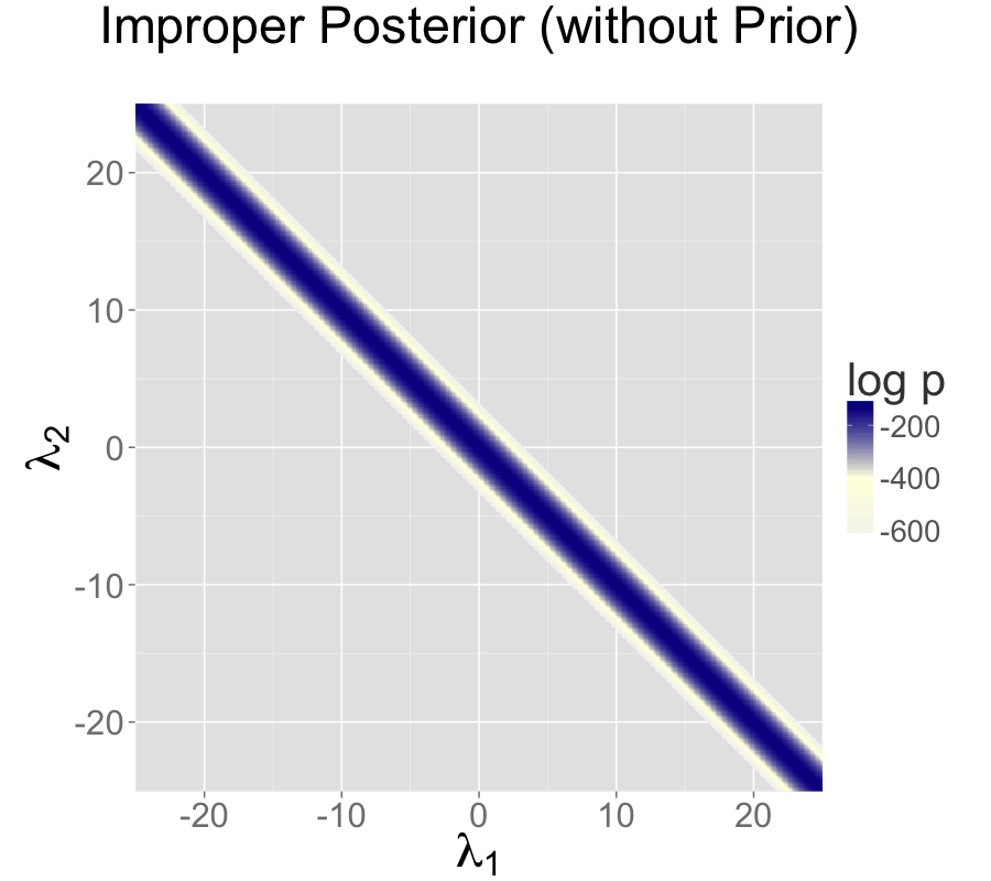
Two intercepts with improper prior
Adding a standard normal prior for the intercepts results in a proper posterior.
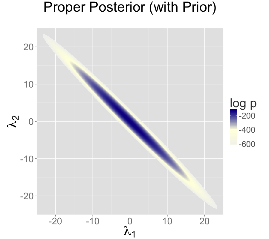
Two intercepts with proper prior
The single intercept parameterization with no prior also has a proper posterior.
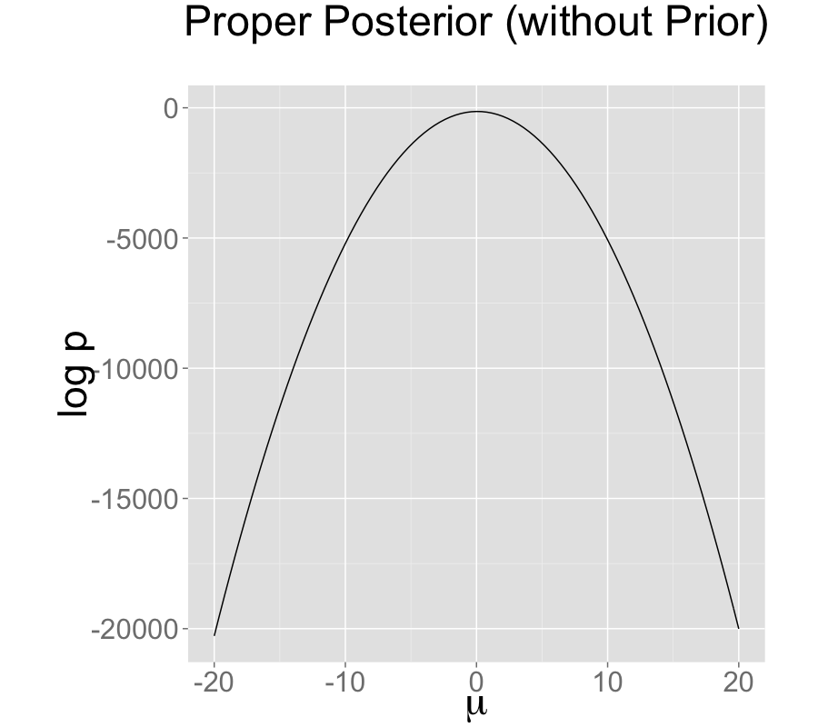
Single intercepts with improper prior
The addition of a prior to the two intercepts model is shown in the second plot; the final plot shows the result of reparameterizing to a single intercept.
An alternative strategy for identifying a \(K\)-simplex parameterization \(\theta = \texttt{softmax}(\alpha)\) in terms of an unconstrained \(K\)-vector \(\alpha\) is to place a prior on the components of \(\alpha\) with a fixed location (that is, specifically avoid hierarchical priors with varying location). Unlike the approaching of pinning \(\alpha_K = 0\), the prior-based approach models the \(K\) outcomes symmetrically rather than modeling \(K-1\) outcomes relative to the \(K\)-th. The pinned parameterization, on the other hand, is usually more efficient statistically because it does not have the extra degree of (prior constrained) wiggle room.
Vague, Strongly Informative, and Weakly Informative Priors
Care must be used when adding a prior to resolve invariances. If the prior is taken to be too broad (i.e., too vague), the resolution is in theory only, and samplers will still struggle.
Ideally, a realistic prior will be formulated based on substantive knowledge of the problem being modeled. Such a prior can be chosen to have the appropriate strength based on prior knowledge. A strongly informative prior makes sense if there is strong prior information.
When there is not strong prior information, a weakly informative prior strikes the proper balance between controlling computational inference without dominating the data in the posterior. In most problems, the modeler will have at least some notion of the expected scale of the estimates and be able to choose a prior for identification purposes that does not dominate the data, but provides sufficient computational control on the posterior.
Priors can also be used in the same way to control the additive invariance of the IRT model. A typical approach is to place a strong prior on student ability parameters \(\alpha\) to control scale simply to control the additive invariance of the basic IRT model and the multiplicative invariance of the model extended with a item discrimination parameters; such a prior does not add any prior knowledge to the problem. Then a prior on item difficulty can be chosen that is either informative or weakly informative based on prior knowledge of the problem.
This example was raised by Richard McElreath on the Stan users group in a query about the difference in behavior between Gibbs sampling as used in BUGS and JAGS and the Hamiltonian Monte Carlo (HMC) and no-U-turn samplers (NUTS) used by Stan.↩︎
The marginal posterior \(p(\sigma \mid y)\) for \(\sigma\) is proper here as long as there are at least two distinct data points.↩︎
A Laplace prior (or an L1 regularizer for penalized maximum likelihood estimation) is not sufficient to remove this additive invariance. It provides shrinkage, but does not in and of itself identify the parameters because adding a constant to \(\lambda_1\) and subtracting it from \(\lambda_2\) results in the same value for the prior density.↩︎