
Extract draws or point estimates from fitted model objects using formats provided by the posterior package. Depending on the fitting method, these are posterior draws from MCMC, approximate posterior draws from variational inference, Laplace approximation, or Pathfinder, standalone generated quantities, or a point estimate from optimization.
The variables include the parameters, transformed parameters, and
generated quantities from the Stan program as well as lp__, the
target log density evaluated by Stan, up to an additive constant. See
$lp() for details.
Usage
draws(
  variables = NULL,
  inc_warmup = FALSE,
  format = getOption("cmdstanr_draws_format")
)
Arguments
- variables
(character vector) Optionally, the names of the variables (parameters, transformed parameters, and generated quantities) to read in.
If
NULL(the default) then all variables are included.If an empty string (
variables="") then none are included.For non-scalar variables all elements or specific elements can be selected:
variables = "theta"selects all elements oftheta;variables = c("theta[1]", "theta[3]")selects only the 1st and 3rd elements.
- inc_warmup
(logical) Should warmup draws be included? Defaults to
FALSE. Ignored except when used with CmdStanMCMC objects.- format
(string) The format of the returned draws or point estimates. Must be a valid format from the posterior package. The defaults are the following.
For sampling and generated quantities the default is
"draws_array". This format keeps the chains separate. To combine the chains use any of the other formats (e.g."draws_matrix").For point estimates from optimization and approximate draws from variational inference, Laplace approximation, and Pathfinder the default is
"draws_matrix".
To use a different format it can be specified as the full name of the format from the posterior package (e.g.
format = "draws_df") or omitting the"draws_"prefix (e.g.format = "df").Changing the default format: To change the default format for an entire R session use
options(cmdstanr_draws_format = format), whereformatis the name (in quotes) of a valid format from the posterior package. For exampleoptions(cmdstanr_draws_format = "draws_df")will change the default to a data frame.Note about efficiency: for sampling and generated quantities,
"draws_array"is the format the draws are read into, so it is the cheapest in time and memory. The other formats are converted from it and need at least one more copy of the draws,"draws_list"and"draws_df"the most. To save memory read only the variables you need with thevariablesargument.
Value
Depends on the value of format. The defaults are:
For MCMC, a 3-D
draws_arrayobject (iteration x chain x variable).For standalone generated quantities, a 3-D
draws_arrayobject (iteration x chain x variable).For variational inference and Laplace approximation, a 2-D
draws_matrixobject (draw x variable). An additional variablelp_approx__containing the log density of the corresponding approximation is also included.For Pathfinder, a 2-D
draws_matrixobject (draw x variable). Additional variableslp_approx__andpath__are also included, withpath__identifying the path associated with each draw.For optimization, a 1-row
draws_matrixwith one column per variable. These are not actually draws, just point estimates stored in thedraws_matrixformat. See$mle()to extract them as a numeric vector.
Examples
# \dontrun{
# logistic regression with intercept alpha and coefficients beta
fit <- cmdstanr_example("logistic", method = "sample")
# returned as 3-D array (see ?posterior::draws_array)
draws <- fit$draws()
dim(draws)
#> [1] 1000 4 105
str(draws)
#> 'draws_array' num [1:1000, 1:4, 1:105] -65.1 -64.7 -64.7 -65.3 -65.3 ...
#> - attr(*, "dimnames")=List of 3
#> ..$ iteration: chr [1:1000] "1" "2" "3" "4" ...
#> ..$ chain : chr [1:4] "1" "2" "3" "4"
#> ..$ variable : chr [1:105] "lp__" "alpha" "beta[1]" "beta[2]" ...
# can easily convert to other formats (data frame, matrix, list)
# using the posterior package
head(posterior::as_draws_matrix(draws))
#> # A draws_matrix: 6 iterations, 1 chains, and 105 variables
#> variable
#> draw lp__ alpha beta[1] beta[2] beta[3] log_lik[1] log_lik[2] log_lik[3]
#> 1 -65 0.42 -0.29 -0.222 0.66 -0.54 -0.46 -0.50
#> 2 -65 0.30 -0.90 -0.164 0.76 -0.50 -0.28 -0.35
#> 3 -65 0.39 -0.65 -0.274 0.34 -0.48 -0.57 -0.52
#> 4 -65 0.27 -0.55 -0.061 0.28 -0.52 -0.52 -0.43
#> 5 -65 0.12 -0.86 -0.419 0.70 -0.61 -0.29 -0.64
#> 6 -64 0.30 -0.65 -0.091 0.56 -0.52 -0.38 -0.38
#> # ... with 97 more variables
# or can specify 'format' argument to avoid manual conversion
# matrix format combines all chains
draws <- fit$draws(format = "matrix")
head(draws)
#> # A draws_matrix: 6 iterations, 1 chains, and 105 variables
#> variable
#> draw lp__ alpha beta[1] beta[2] beta[3] log_lik[1] log_lik[2] log_lik[3]
#> 1 -65 0.42 -0.29 -0.222 0.66 -0.54 -0.46 -0.50
#> 2 -65 0.30 -0.90 -0.164 0.76 -0.50 -0.28 -0.35
#> 3 -65 0.39 -0.65 -0.274 0.34 -0.48 -0.57 -0.52
#> 4 -65 0.27 -0.55 -0.061 0.28 -0.52 -0.52 -0.43
#> 5 -65 0.12 -0.86 -0.419 0.70 -0.61 -0.29 -0.64
#> 6 -64 0.30 -0.65 -0.091 0.56 -0.52 -0.38 -0.38
#> # ... with 97 more variables
# can select specific parameters
fit$draws("alpha")
#> # A draws_array: 1000 iterations, 4 chains, and 1 variables
#> , , variable = alpha
#>
#> chain
#> iteration 1 2 3 4
#> 1 0.42 0.10 0.28 0.33
#> 2 0.30 0.41 0.40 0.15
#> 3 0.39 0.33 0.65 0.43
#> 4 0.27 0.40 0.12 0.15
#> 5 0.12 0.16 0.54 0.23
#>
#> # ... with 995 more iterations
fit$draws("beta") # selects entire vector beta
#> # A draws_array: 1000 iterations, 4 chains, and 3 variables
#> , , variable = beta[1]
#>
#> chain
#> iteration 1 2 3 4
#> 1 -0.29 -0.86 -0.81 -0.64
#> 2 -0.90 -0.70 -0.46 -0.63
#> 3 -0.65 -0.54 -0.96 -0.78
#> 4 -0.55 -0.94 -0.50 -1.25
#> 5 -0.86 -0.89 -0.98 -0.63
#>
#> , , variable = beta[2]
#>
#> chain
#> iteration 1 2 3 4
#> 1 -0.222 -0.32 -0.27 -0.352
#> 2 -0.164 -0.50 -0.43 -0.025
#> 3 -0.274 -0.53 -0.31 -0.276
#> 4 -0.061 -0.17 -0.23 -0.372
#> 5 -0.419 -0.51 -0.30 0.016
#>
#> , , variable = beta[3]
#>
#> chain
#> iteration 1 2 3 4
#> 1 0.66 0.46 0.58 0.62
#> 2 0.76 0.91 0.71 0.66
#> 3 0.34 0.81 0.86 0.66
#> 4 0.28 0.67 0.45 0.57
#> 5 0.70 0.58 0.35 0.22
#>
#> # ... with 995 more iterations
fit$draws(c("alpha", "beta[2]"))
#> # A draws_array: 1000 iterations, 4 chains, and 2 variables
#> , , variable = alpha
#>
#> chain
#> iteration 1 2 3 4
#> 1 0.42 0.10 0.28 0.33
#> 2 0.30 0.41 0.40 0.15
#> 3 0.39 0.33 0.65 0.43
#> 4 0.27 0.40 0.12 0.15
#> 5 0.12 0.16 0.54 0.23
#>
#> , , variable = beta[2]
#>
#> chain
#> iteration 1 2 3 4
#> 1 -0.222 -0.32 -0.27 -0.352
#> 2 -0.164 -0.50 -0.43 -0.025
#> 3 -0.274 -0.53 -0.31 -0.276
#> 4 -0.061 -0.17 -0.23 -0.372
#> 5 -0.419 -0.51 -0.30 0.016
#>
#> # ... with 995 more iterations
# can be passed directly to bayesplot plotting functions
bayesplot::color_scheme_set("brightblue")
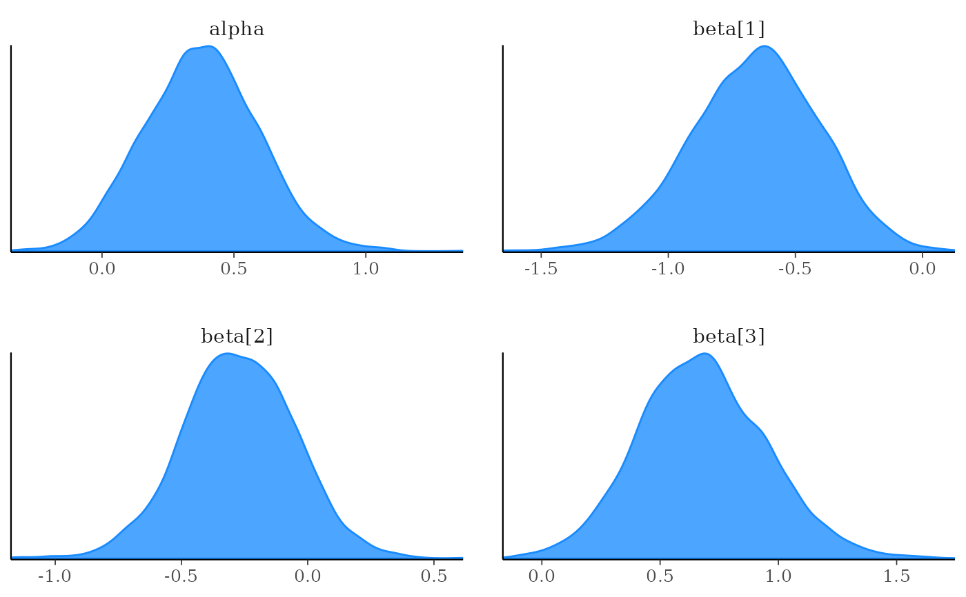
bayesplot::mcmc_dens(fit$draws(c("alpha", "beta")))
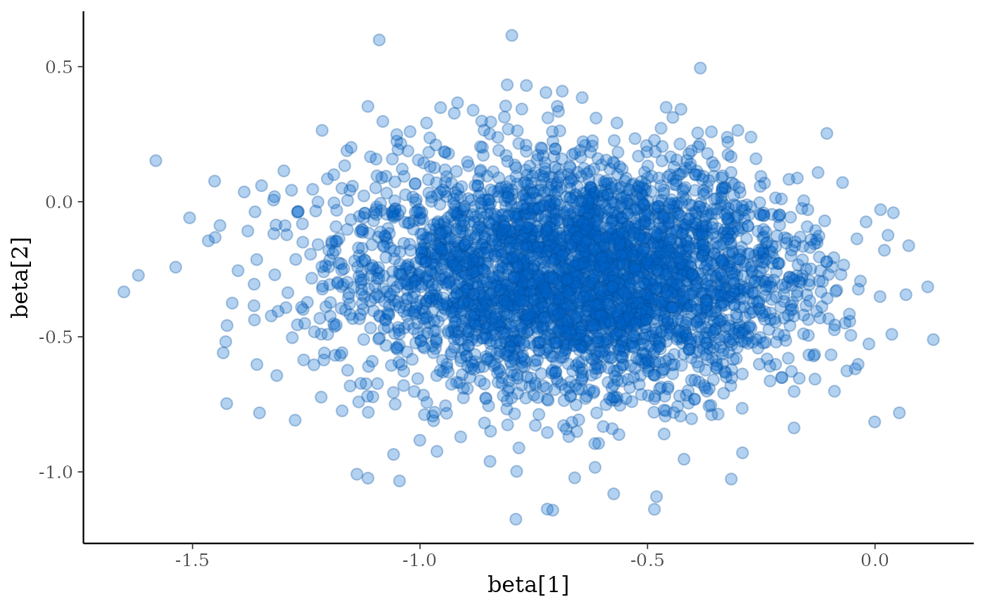
 bayesplot::mcmc_scatter(fit$draws(c("beta[1]", "beta[2]")), alpha = 0.3)
 # example using variational inference
fit <- cmdstanr_example("logistic", method = "variational")
head(fit$draws("beta")) # a matrix by default
#> # A draws_matrix: 6 iterations, 1 chains, and 3 variables
#> variable
#> draw beta[1] beta[2] beta[3]
#> 1 -0.43 -0.509 0.34
#> 2 -0.58 0.087 0.36
#> 3 -0.34 -0.209 0.46
#> 4 -0.91 -0.689 1.26
#> 5 -0.47 -0.349 0.66
#> 6 -0.35 -0.314 0.93
head(fit$draws("beta", format = "df"))
#> # A draws_df: 6 iterations, 1 chains, and 3 variables
#> beta[1] beta[2] beta[3]
#> 1 -0.43 -0.509 0.34
#> 2 -0.58 0.087 0.36
#> 3 -0.34 -0.209 0.46
#> 4 -0.91 -0.689 1.26
#> 5 -0.47 -0.349 0.66
#> 6 -0.35 -0.314 0.93
#> # ... hidden reserved variables {'.chain', '.iteration', '.draw'}
# }
# example using variational inference
fit <- cmdstanr_example("logistic", method = "variational")
head(fit$draws("beta")) # a matrix by default
#> # A draws_matrix: 6 iterations, 1 chains, and 3 variables
#> variable
#> draw beta[1] beta[2] beta[3]
#> 1 -0.43 -0.509 0.34
#> 2 -0.58 0.087 0.36
#> 3 -0.34 -0.209 0.46
#> 4 -0.91 -0.689 1.26
#> 5 -0.47 -0.349 0.66
#> 6 -0.35 -0.314 0.93
head(fit$draws("beta", format = "df"))
#> # A draws_df: 6 iterations, 1 chains, and 3 variables
#> beta[1] beta[2] beta[3]
#> 1 -0.43 -0.509 0.34
#> 2 -0.58 0.087 0.36
#> 3 -0.34 -0.209 0.46
#> 4 -0.91 -0.689 1.26
#> 5 -0.47 -0.349 0.66
#> 6 -0.35 -0.314 0.93
#> # ... hidden reserved variables {'.chain', '.iteration', '.draw'}
# }