PPD intervals

Medians and central interval estimates of posterior or prior predictive distributions. Each of these functions makes the same plot as the corresponding ppc_ function but without plotting any observed data y. The Plot Descriptions section at PPC-intervals has details on the individual plots.

Usage

ppd_intervals(
  ypred,
  x = NULL,
  ...,
  prob = 0.5,
  prob_outer = 0.9,
  alpha = 0.33,
  size = 1,
  fatten = 2.5,
  linewidth = 1
)

ppd_intervals_grouped(
  ypred,
  x = NULL,
  group,
  ...,
  facet_args = list(),
  prob = 0.5,
  prob_outer = 0.9,
  alpha = 0.33,
  size = 1,
  fatten = 2.5,
  linewidth = 1
)

ppd_ribbon(
  ypred,
  x = NULL,
  ...,
  prob = 0.5,
  prob_outer = 0.9,
  alpha = 0.33,
  size = 0.25
)

ppd_ribbon_grouped(
  ypred,
  x = NULL,
  group,
  ...,
  facet_args = list(),
  prob = 0.5,
  prob_outer = 0.9,
  alpha = 0.33,
  size = 0.25
)

ppd_intervals_data(
  ypred,
  x = NULL,
  group = NULL,
  ...,
  prob = 0.5,
  prob_outer = 0.9
)

ppd_ribbon_data(
  ypred,
  x = NULL,
  group = NULL,
  ...,
  prob = 0.5,
  prob_outer = 0.9
)

Arguments

ypred

An S by N matrix of draws from the posterior (or prior) predictive distribution, or a posterior::draws object. The number of rows, S, is the size of the posterior (or prior) sample used to generate ypred. The number of columns, N, is the number of predicted observations.

x

A numeric vector to use as the x-axis variable. For example, x could be a predictor variable from a regression model, a time variable for time-series models, etc. If x is missing or NULL then the observation index is used for the x-axis.

...

Currently unused.

prob, prob_outer

Values between 0 and 1 indicating the desired probability mass to include in the inner and outer intervals. The defaults are prob=0.5 and prob_outer=0.9.

alpha, size, fatten, linewidth

Arguments passed to geoms. For ribbon plots alpha is passed to ggplot2::geom_ribbon() to control the opacity of the outer ribbon and size is passed to ggplot2::geom_line() to control the size of the line representing the median prediction (size=0 will remove the line). For interval plots alpha, size, fatten, and linewidth are passed to ggplot2::geom_pointrange() (fatten=0 will remove the point estimates).

group

A grouping variable of the same length as y. Will be coerced to factor if not already a factor. Each value in group is interpreted as the group level pertaining to the corresponding observation.

facet_args

A named list of arguments (other than facets) passed to ggplot2::facet_wrap() or ggplot2::facet_grid() to control faceting. Note: if scales is not included in facet_args then bayesplot may use scales="free" as the default (depending on the plot) instead of the ggplot2 default of scales="fixed".

Value

The plotting functions return a ggplot object that can be further customized using the ggplot2 package. The functions with suffix _data() return the data that would have been drawn by the plotting function.

References

Gabry, J. , Simpson, D. , Vehtari, A. , Betancourt, M. and Gelman, A. (2019), Visualization in Bayesian workflow. J. R. Stat. Soc. A, 182: 389-402. doi:10.1111/rssa.12378. (journal version, arXiv preprint, code on GitHub)

See also

Other PPDs: PPD-distributions, PPD-overview, PPD-test-statistics

Examples

color_scheme_set("brightblue")
ypred <- example_yrep_draws()
x <- example_x_data()
group <- example_group_data()

ppd_intervals(ypred[, 1:50])

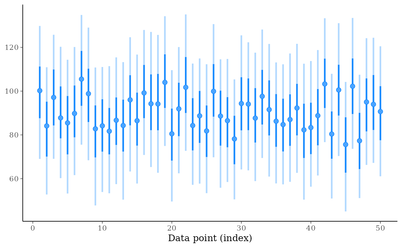ppd_intervals(ypred[, 1:50], fatten = 0)

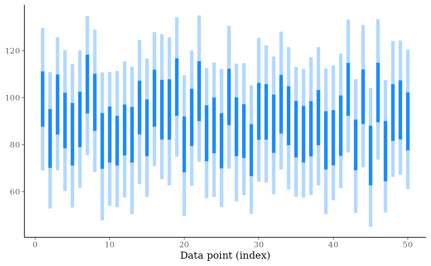
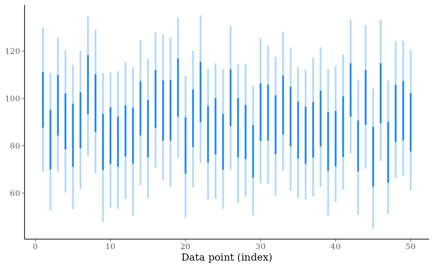ppd_intervals(ypred[, 1:50], fatten = 0, linewidth = 2)

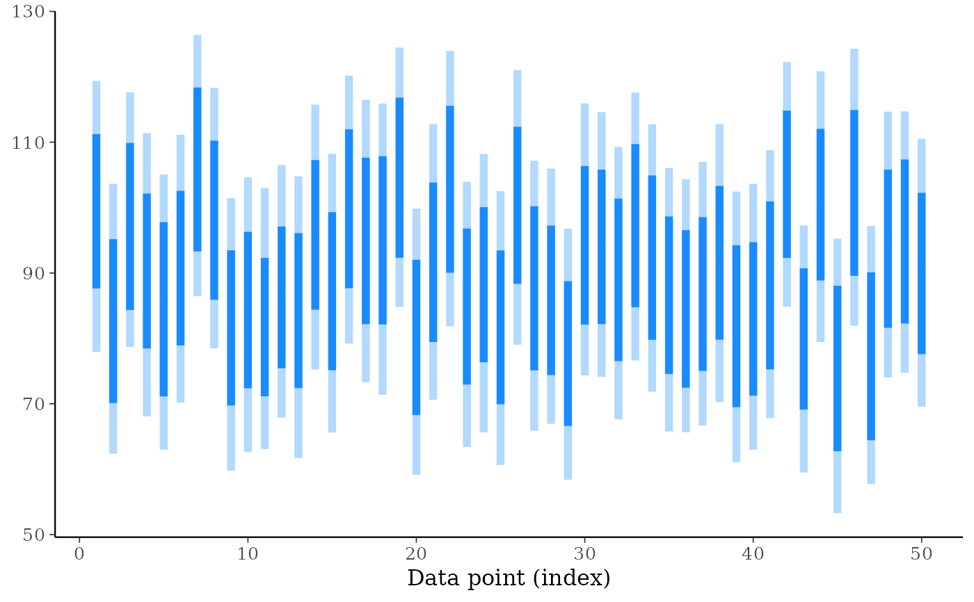
ppd_intervals(ypred[, 1:50], prob_outer = 0.75, fatten = 0, linewidth = 2)


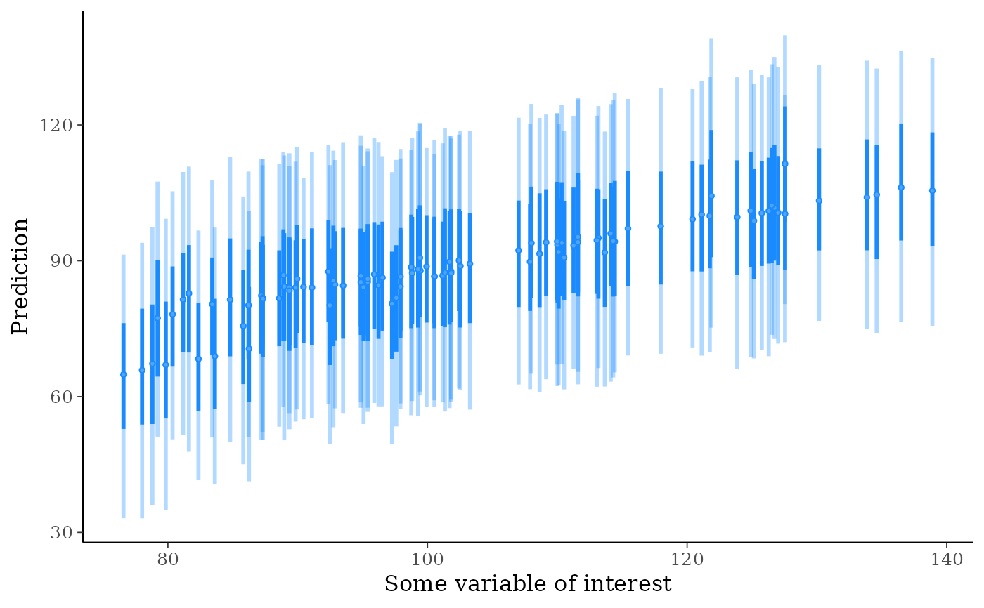
# put a predictor variable on the x-axis
ppd_intervals(ypred[, 1:100], x = x[1:100], fatten = 1) +
  ggplot2::labs(y = "Prediction", x = "Some variable of interest")


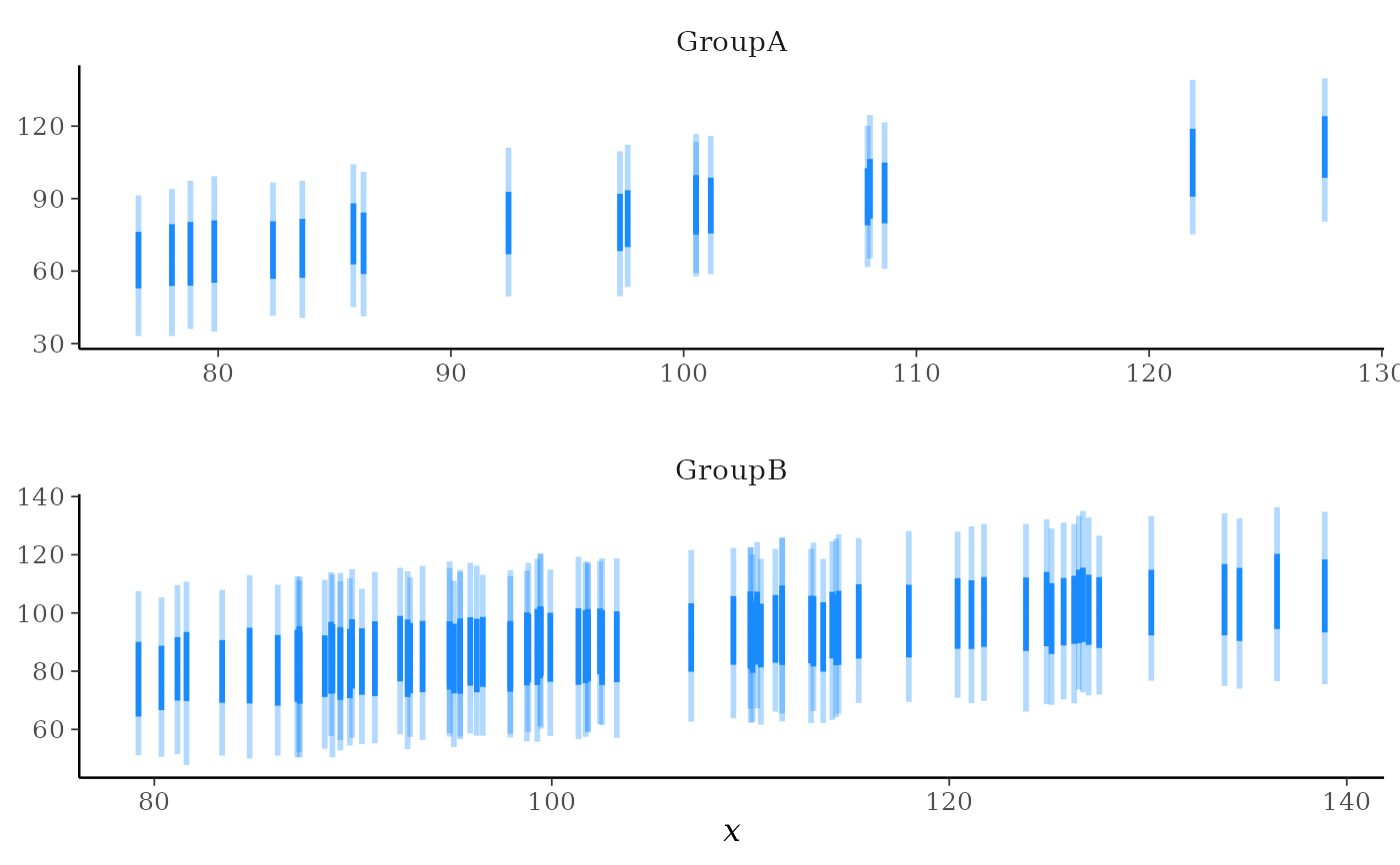
# with a grouping variable too
ppd_intervals_grouped(
  ypred = ypred[, 1:100],
  x = x[1:100],
  group = group[1:100],
  size = 2,
  fatten = 0,
  facet_args = list(nrow = 2)
)


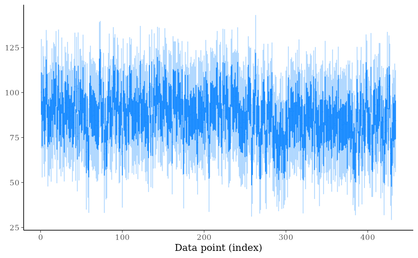
# even reducing size, ppd_intervals is too cluttered when there are many
# observations included (ppd_ribbon is better)
ppd_intervals(ypred, size = 0.5, fatten = 0.1, linewidth = 0.5)

ppd_ribbon(ypred)

ppd_ribbon(ypred, size = 0) # remove line showing median prediction