PPD distributions

Plot posterior or prior predictive distributions. Each of these functions makes the same plot as the corresponding ppc_ function but without plotting any observed data y. The Plot Descriptions section at PPC-distributions has details on the individual plots.

Usage

ppd_data(ypred, group = NULL)

ppd_dens_overlay(
  ypred,
  show_marginal = FALSE,
  ...,
  size = 0.25,
  alpha = 0.7,
  trim = FALSE,
  bw = NULL,
  adjust = NULL,
  kernel = NULL,
  bounds = NULL,
  n_dens = NULL
)

ppd_ecdf_overlay(
  ypred,
  show_marginal = FALSE,
  ...,
  discrete = deprecated(),
  pad = TRUE,
  size = 0.25,
  alpha = 0.7
)

ppd_dens(
  ypred,
  show_marginal = FALSE,
  ...,
  trim = FALSE,
  size = 0.5,
  alpha = 1,
  bounds = NULL
)

ppd_hist(
  ypred,
  show_marginal = FALSE,
  ...,
  binwidth = NULL,
  bins = NULL,
  breaks = NULL,
  freq = !show_marginal
)

ppd_dots(
  ypred,
  show_marginal = FALSE,
  ...,
  binwidth = NA,
  quantiles = 100,
  freq = TRUE
)

ppd_freqpoly(
  ypred,
  show_marginal = FALSE,
  ...,
  binwidth = NULL,
  bins = NULL,
  freq = !show_marginal,
  size = 0.5,
  alpha = 1
)

ppd_freqpoly_grouped(
  ypred,
  group,
  show_marginal = FALSE,
  ...,
  binwidth = NULL,
  bins = NULL,
  freq = !show_marginal,
  size = 0.5,
  alpha = 1
)

ppd_boxplot(
  ypred,
  show_marginal = FALSE,
  ...,
  notch = TRUE,
  size = 0.5,
  alpha = 1
)

Arguments

ypred

An S by N matrix of draws from the posterior (or prior) predictive distribution, or a posterior::draws object. The number of rows, S, is the size of the posterior (or prior) sample used to generate ypred. The number of columns, N, is the number of predicted observations.

group

A grouping variable of the same length as y. Will be coerced to factor if not already a factor. Each value in group is interpreted as the group level pertaining to the corresponding observation.

show_marginal

Plot the marginal PPD along with the ypreds.

...

For dot plots, optional additional arguments to pass to ggdist::stat_dots().

size, alpha

Passed to the appropriate geom to control the appearance of the predictive distributions.

trim

A logical scalar passed to ggplot2::geom_density().

bw, adjust, kernel, n_dens, bounds

Optional arguments passed to stats::density() (and bounds to ggplot2::stat_density()) to override default kernel density estimation parameters or truncate the density support. If NULL (default), bw is set to "nrd0", adjust to 1, kernel to "gaussian", and n_dens to 1024.

discrete

The discrete argument is deprecated. The ECDF is a step function by definition, so geom_step() is now always used.

pad

A logical scalar passed to ggplot2::stat_ecdf().

binwidth

Passed to ggplot2::geom_histogram(), ggplot2::geom_area(), and ggdist::stat_dots() to override the default binwidth.

bins

Passed to ggplot2::geom_histogram() and ggplot2::geom_area() to override the default binning.

breaks

Passed to ggplot2::geom_histogram() as an alternative to binwidth.

freq

For histograms and frequency polygons, freq=TRUE (the default) puts count on the y-axis. Setting freq=FALSE puts density on the y-axis. (For many plots the y-axis text is off by default. To view the count or density labels on the y-axis see the yaxis_text() convenience function.)

quantiles

For dot plots, an optional integer passed to ggdist::stat_dots() specifying the number of quantiles to use for a quantile dot plot. If quantiles is NA then all data points are plotted. The default is quantiles=100 so that each dot represent one percent of posterior mass.

notch

For the box plot, a logical scalar passed to ggplot2::geom_boxplot(). Note: unlike geom_boxplot(), the default is notch=TRUE.

Value

The plotting functions return a ggplot object that can be further customized using the ggplot2 package. The functions with suffix _data() return the data that would have been drawn by the plotting function.

Details

For Binomial data, the plots may be more useful if the input contains the "success" proportions (not discrete "success" or "failure" counts).

See also

Other PPDs: PPD-intervals, PPD-overview, PPD-test-statistics

Examples

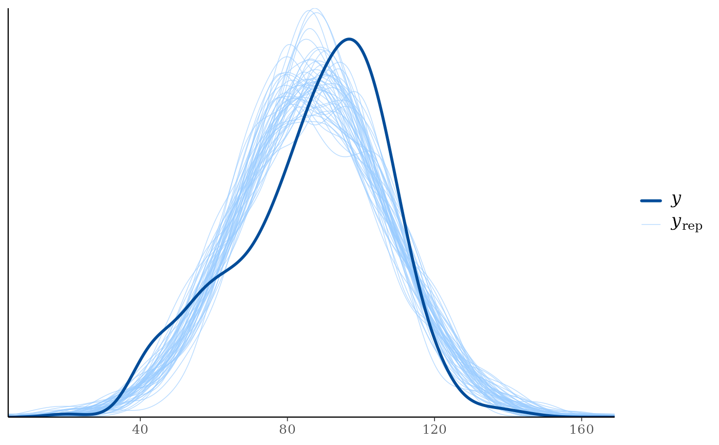
# difference between ppd_dens_overlay() and ppc_dens_overlay()
color_scheme_set("brightblue")
preds <- example_yrep_draws()
ppd_dens_overlay(ypred = preds[1:50, ])

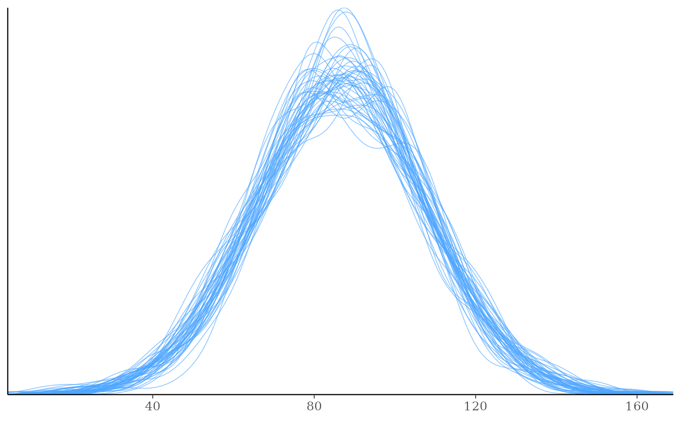ppd_dens_overlay(ypred = preds[1:50, ], show_marginal = TRUE)

ppc_dens_overlay(y = example_y_data(), yrep = preds[1:50, ])