Plot central (quantile-based) posterior interval estimates from MCMC draws. See the Plot Descriptions section, below, for details.
Usage
mcmc_intervals(
  x,
  pars = character(),
  regex_pars = character(),
  transformations = list(),
  ...,
  prob = 0.5,
  prob_outer = 0.9,
  point_est = c("median", "mean", "none"),
  outer_size = 0.5,
  inner_size = 2,
  point_size = 4,
  rhat = numeric()
)

mcmc_areas(
  x,
  pars = character(),
  regex_pars = character(),
  transformations = list(),
  ...,
  area_method = c("equal area", "equal height", "scaled height"),
  prob = 0.5,
  prob_outer = 1,
  point_est = c("median", "mean", "none"),
  rhat = numeric(),
  border_size = NULL,
  bw = NULL,
  adjust = NULL,
  kernel = NULL,
  n_dens = NULL,
  bounds = NULL
)

mcmc_areas_ridges(
  x,
  pars = character(),
  regex_pars = character(),
  transformations = list(),
  ...,
  prob_outer = 1,
  prob = 1,
  border_size = NULL,
  bw = NULL,
  adjust = NULL,
  kernel = NULL,
  n_dens = NULL,
  bounds = NULL
)

mcmc_intervals_data(
  x,
  pars = character(),
  regex_pars = character(),
  transformations = list(),
  ...,
  prob = 0.5,
  prob_outer = 0.9,
  point_est = c("median", "mean", "none"),
  rhat = numeric()
)

mcmc_areas_data(
  x,
  pars = character(),
  regex_pars = character(),
  transformations = list(),
  ...,
  prob = 0.5,
  prob_outer = 1,
  point_est = c("median", "mean", "none"),
  rhat = numeric(),
  bw = NULL,
  adjust = NULL,
  kernel = NULL,
  n_dens = NULL,
  bounds = NULL
)

mcmc_areas_ridges_data(
  x,
  pars = character(),
  regex_pars = character(),
  transformations = list(),
  ...,
  prob_outer = 1,
  prob = 1,
  bw = NULL,
  adjust = NULL,
  kernel = NULL,
  n_dens = NULL,
  bounds = NULL
)
Arguments
- x
An object containing MCMC draws:
A 3-D array, matrix, list of matrices, or data frame. The MCMC-overview page provides details on how to specify each these.
A
drawsobject from the posterior package (e.g.,draws_array,draws_rvars, etc.).An object with an
as.array()method that returns the same kind of 3-D array described on the MCMC-overview page.
- pars
An optional character vector of parameter names. If neither
parsnorregex_parsis specified then the default is to use all parameters. As of version1.7.0, bayesplot also supports 'tidy' parameter selection by specifyingpars = vars(...), where...is specified the same way as in dplyr::select(...) and similar functions. Examples of usingparsin this way can be found on the Tidy parameter selection page.- regex_pars
An optional regular expression to use for parameter selection. Can be specified instead of
parsor in addition topars. When usingparsfor tidy parameter selection, theregex_parsargument is ignored since select helpers perform a similar function.- transformations
Optionally, transformations to apply to parameters before plotting. If
transformationsis a function or a single string naming a function then that function will be used to transform all parameters. To apply transformations to particular parameters, thetransformationsargument can be a named list with length equal to the number of parameters to be transformed. Currently only univariate transformations of scalar parameters can be specified (multivariate transformations will be implemented in a future release). Iftransformationsis a list, the name of each list element should be a parameter name and the content of each list element should be a function (or any item to match as a function viamatch.fun(), e.g. a string naming a function). If a function is specified by its name as a string (e.g."log"), then it can be used to construct a new parameter label for the appropriate parameter (e.g."log(sigma)"). If a function itself is specified (e.g.logorfunction(x) log(x)) then"t"is used in the new parameter label to indicate that the parameter is transformed (e.g."t(sigma)").Note: due to partial argument matching
transformationscan be abbreviated for convenience in interactive use (e.g.,transform).- ...
Currently unused.
- prob
The probability mass to include in the inner interval (for
mcmc_intervals()) or in the shaded region (formcmc_areas()). The default is0.5(50% interval) and1formcmc_areas_ridges().- prob_outer
The probability mass to include in the outer interval. The default is
0.9formcmc_intervals()(90% interval) and1formcmc_areas()and formcmc_areas_ridges().- point_est
The point estimate to show. Either
"median"(the default),"mean", or"none".- inner_size, outer_size
For
mcmc_intervals(), the size of the inner and interval segments, respectively.- point_size
For
mcmc_intervals(), the size of point estimate.- rhat
An optional numeric vector of R-hat estimates, with one element per parameter included in
x. Ifrhatis provided, the intervals/areas and point estimates in the resulting plot are colored based on R-hat value. Seerhat()for methods for extracting R-hat estimates.- area_method
How to constrain the areas in
mcmc_areas(). The default is"equal area", setting the density curves to have the same area. With"equal height", the curves are scaled so that the highest points across the curves are the same height. The method"scaled height"tries a compromise between to the two: the heights from"equal height"are scaled usingheight*sqrt(height)- border_size
For
mcmc_areas()andmcmc_areas_ridges(), the size of the ridgelines.- bw, adjust, kernel, n_dens, bounds
Optional arguments passed to
stats::density()(andboundstoggplot2::stat_density()) to override default kernel density estimation parameters or truncate the density support. IfNULL(default),bwis set to"nrd0",adjustto1,kernelto"gaussian", andn_densto1024.
Value
The plotting functions return a ggplot object that can be further
customized using the ggplot2 package. The functions with suffix
_data() return the data that would have been drawn by the plotting
function.
Plot Descriptions
mcmc_intervals()Plots of uncertainty intervals computed from posterior draws with all chains merged.
mcmc_areas()Density plots computed from posterior draws with all chains merged, with uncertainty intervals shown as shaded areas under the curves.
mcmc_areas_ridges()Density plot, as in
mcmc_areas(), but drawn with overlapping ridgelines. This plot provides a compact display of (hierarchically) related distributions.mcmc_intervals_data(),mcmc_areas_data(),mcmc_areas_ridges_data()Data-preparation back ends for
mcmc_intervals(),mcmc_areas(), andmcmc_areas_ridges(), respectively. Users can call these functions directly to obtain the prepared data frames of posterior interval summaries and create custom interval or density-area visualizations with ggplot2.
Examples
set.seed(9262017)
# load ggplot2 to use its functions to modify our plots
library(ggplot2)
# some parameter draws to use for demonstration
x <- example_mcmc_draws(params = 6)
dim(x)
#> [1] 250 4 6
dimnames(x)
#> $Iteration
#> NULL
#>
#> $Chain
#> [1] "chain:1" "chain:2" "chain:3" "chain:4"
#>
#> $Parameter
#> [1] "alpha" "sigma" "beta[1]" "beta[2]" "beta[3]" "beta[4]"
#>
color_scheme_set("brightblue")
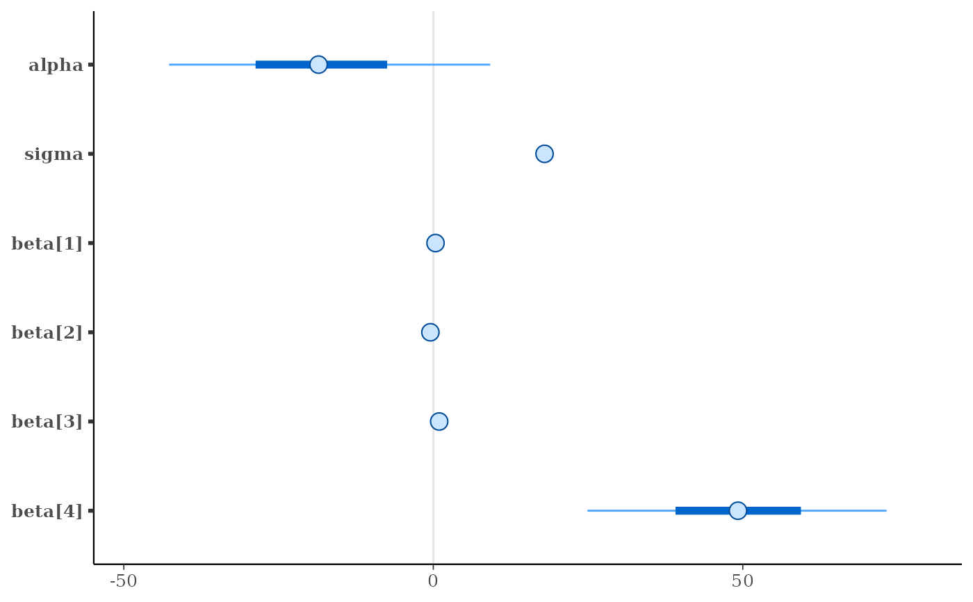
mcmc_intervals(x)
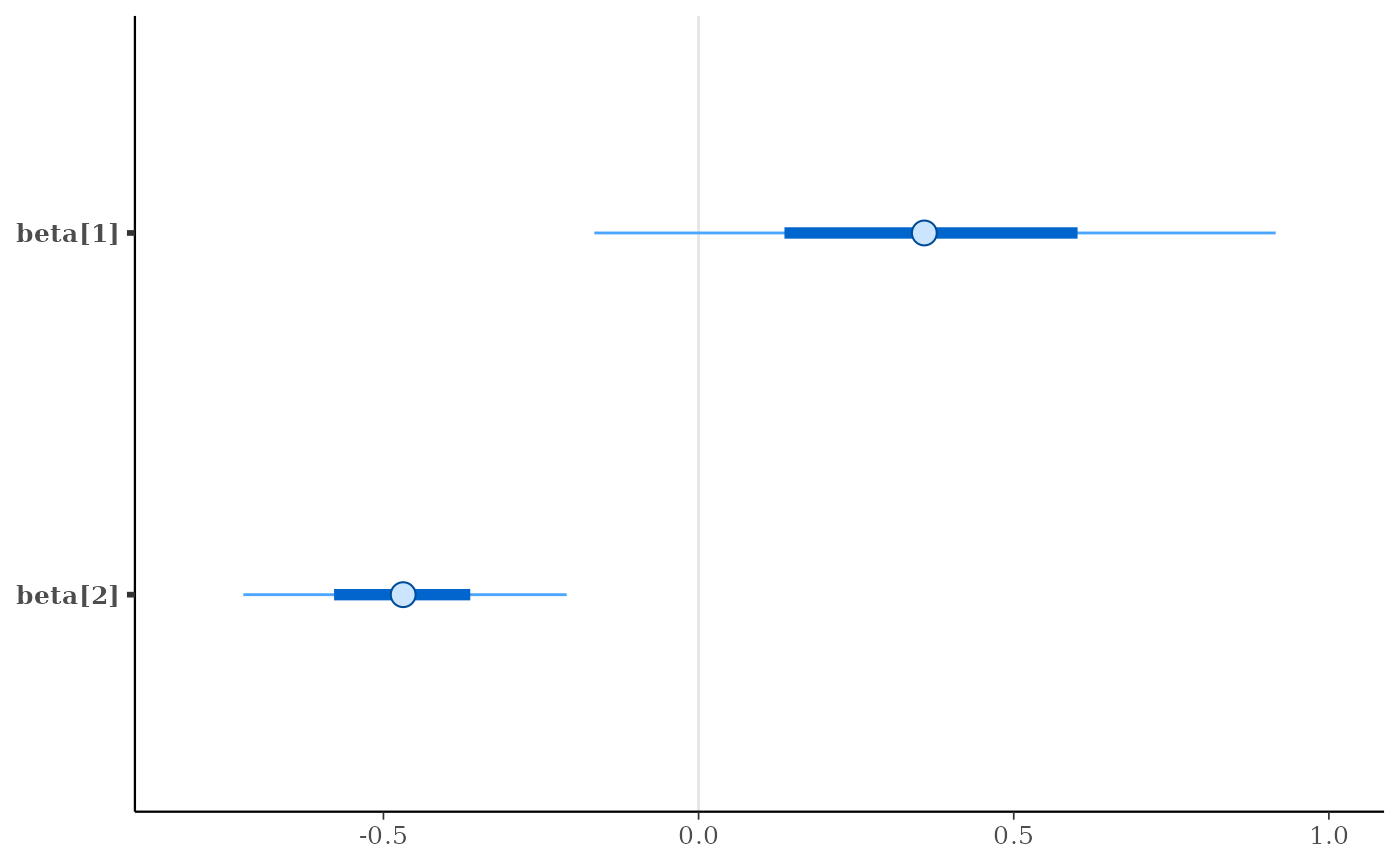
 mcmc_intervals(x, pars = c("beta[1]", "beta[2]"))
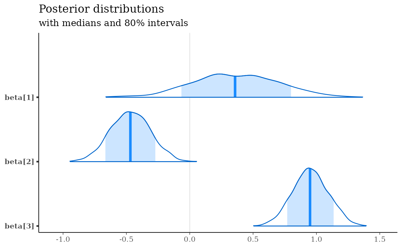
 mcmc_areas(x, regex_pars = "beta\\[[1-3]\\]", prob = 0.8) +
labs(
title = "Posterior distributions",
subtitle = "with medians and 80% intervals"
)
mcmc_areas(x, regex_pars = "beta\\[[1-3]\\]", prob = 0.8) +
labs(
title = "Posterior distributions",
subtitle = "with medians and 80% intervals"
)
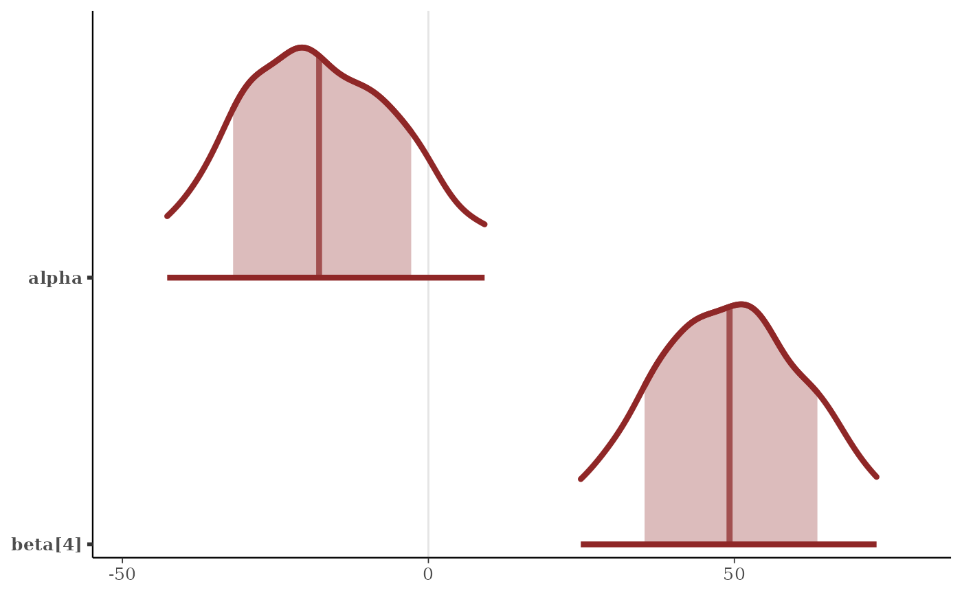
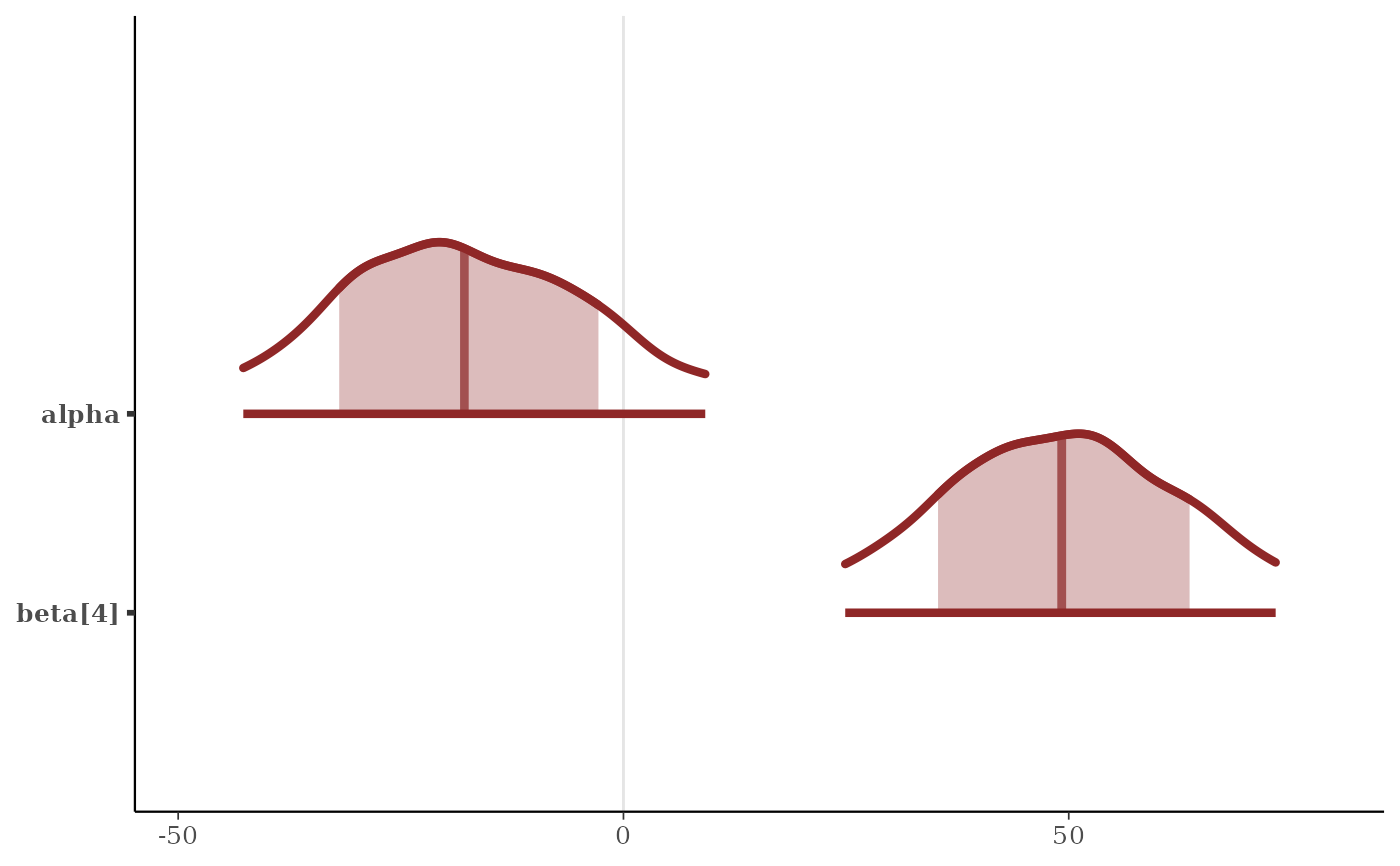
 color_scheme_set("red")
p <- mcmc_areas(
x,
pars = c("alpha", "beta[4]"),
prob = 2/3,
prob_outer = 0.9,
point_est = "mean",
border_size = 1.5 # make the ridgelines fatter
)
plot(p)
color_scheme_set("red")
p <- mcmc_areas(
x,
pars = c("alpha", "beta[4]"),
prob = 2/3,
prob_outer = 0.9,
point_est = "mean",
border_size = 1.5 # make the ridgelines fatter
)
plot(p)
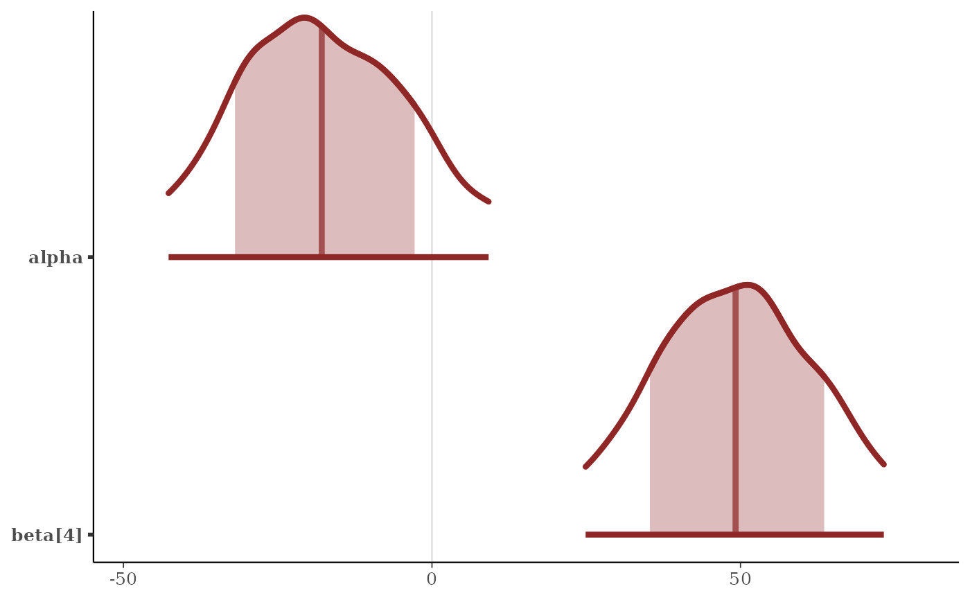
 # \donttest{
# control spacing at top and bottom of plot
# see ?ggplot2::expansion
p + scale_y_discrete(
limits = c("beta[4]", "alpha"),
expand = expansion(add = c(1, 2))
)
#> Scale for y is already present.
#> Adding another scale for y, which will replace the existing scale.
# \donttest{
# control spacing at top and bottom of plot
# see ?ggplot2::expansion
p + scale_y_discrete(
limits = c("beta[4]", "alpha"),
expand = expansion(add = c(1, 2))
)
#> Scale for y is already present.
#> Adding another scale for y, which will replace the existing scale.
 p + scale_y_discrete(
limits = c("beta[4]", "alpha"),
expand = expansion(add = c(.1, .3))
)
#> Scale for y is already present.
#> Adding another scale for y, which will replace the existing scale.
p + scale_y_discrete(
limits = c("beta[4]", "alpha"),
expand = expansion(add = c(.1, .3))
)
#> Scale for y is already present.
#> Adding another scale for y, which will replace the existing scale.
 # relabel parameters
p + scale_y_discrete(
labels = c("alpha" = "param label 1",
"beta[4]" = "param label 2")
)
#> Scale for y is already present.
#> Adding another scale for y, which will replace the existing scale.
# relabel parameters
p + scale_y_discrete(
labels = c("alpha" = "param label 1",
"beta[4]" = "param label 2")
)
#> Scale for y is already present.
#> Adding another scale for y, which will replace the existing scale.
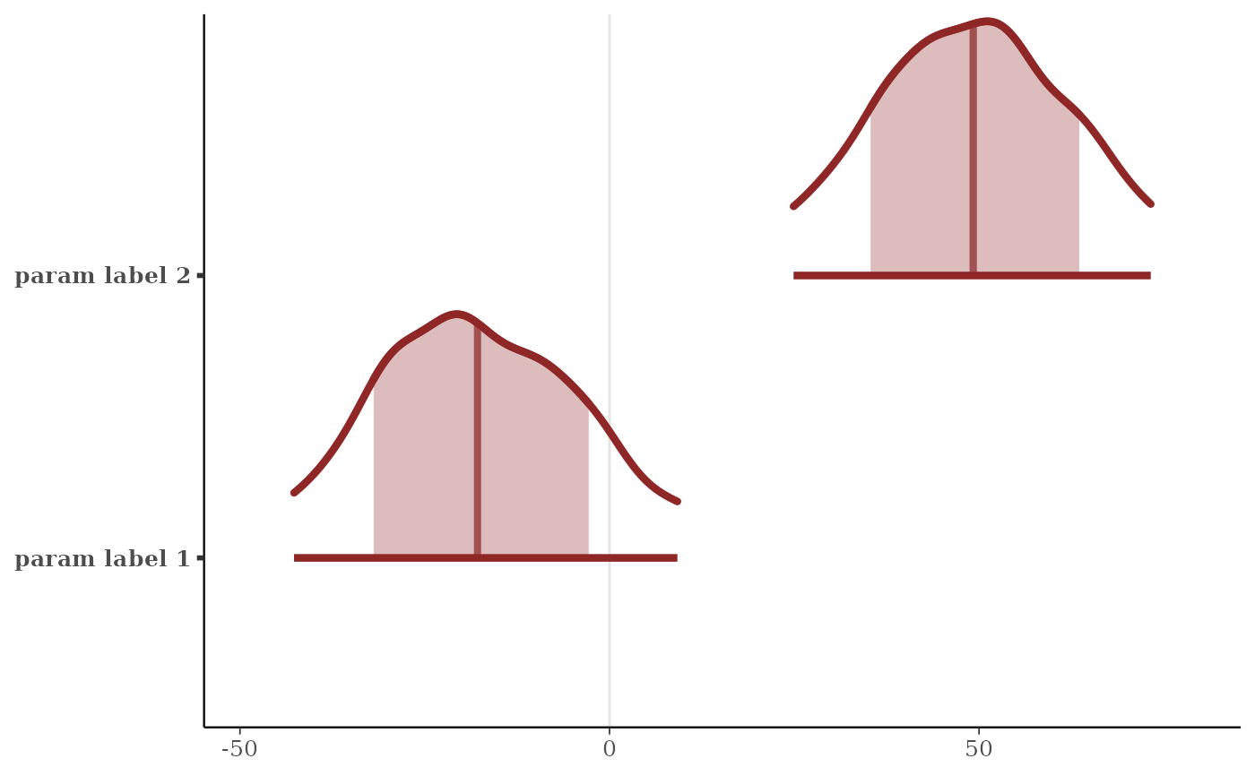 # relabel parameters and define the order
p + scale_y_discrete(
labels = c("alpha" = "param label 1",
"beta[4]" = "param label 2"),
limits = c("beta[4]", "alpha")
)
#> Scale for y is already present.
#> Adding another scale for y, which will replace the existing scale.
# relabel parameters and define the order
p + scale_y_discrete(
labels = c("alpha" = "param label 1",
"beta[4]" = "param label 2"),
limits = c("beta[4]", "alpha")
)
#> Scale for y is already present.
#> Adding another scale for y, which will replace the existing scale.
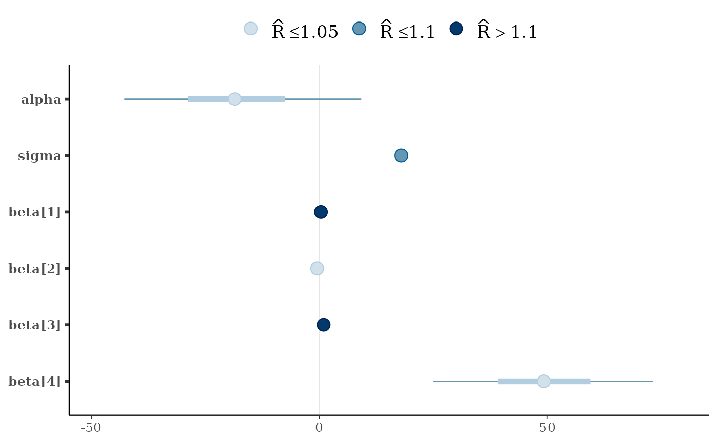
 # color by rhat value
color_scheme_set("blue")
fake_rhat_values <- c(1, 1.07, 1.3, 1.01, 1.15, 1.005)
mcmc_intervals(x, rhat = fake_rhat_values)
# color by rhat value
color_scheme_set("blue")
fake_rhat_values <- c(1, 1.07, 1.3, 1.01, 1.15, 1.005)
mcmc_intervals(x, rhat = fake_rhat_values)
 # get the dataframe that is used in the plotting functions
mcmc_intervals_data(x)
#> # A tibble: 6 × 9
#> parameter outer_width inner_width point_est ll l m h
#> <fct> <dbl> <dbl> <chr> <dbl> <dbl> <dbl> <dbl>
#> 1 alpha 0.9 0.5 median -42.7 -28.7 -18.5 -7.46
#> 2 sigma 0.9 0.5 median 17.1 17.6 18.0 18.4
#> 3 beta[1] 0.9 0.5 median -0.165 0.136 0.358 0.601
#> 4 beta[2] 0.9 0.5 median -0.722 -0.578 -0.469 -0.362
#> 5 beta[3] 0.9 0.5 median 0.718 0.858 0.950 1.05
#> 6 beta[4] 0.9 0.5 median 24.9 39.1 49.2 59.4
#> # ℹ 1 more variable: hh <dbl>
mcmc_intervals_data(x, rhat = fake_rhat_values)
#> # A tibble: 6 × 12
#> parameter outer_width inner_width point_est ll l m h
#> <fct> <dbl> <dbl> <chr> <dbl> <dbl> <dbl> <dbl>
#> 1 alpha 0.9 0.5 median -42.7 -28.7 -18.5 -7.46
#> 2 sigma 0.9 0.5 median 17.1 17.6 18.0 18.4
#> 3 beta[1] 0.9 0.5 median -0.165 0.136 0.358 0.601
#> 4 beta[2] 0.9 0.5 median -0.722 -0.578 -0.469 -0.362
#> 5 beta[3] 0.9 0.5 median 0.718 0.858 0.950 1.05
#> 6 beta[4] 0.9 0.5 median 24.9 39.1 49.2 59.4
#> # ℹ 4 more variables: hh <dbl>, rhat_value <dbl>, rhat_rating <fct>,
#> # rhat_description <chr>
mcmc_areas_data(x, pars = "alpha")
#> # A tibble: 2,091 × 7
#> parameter interval interval_width x density scaled_density
#> <fct> <chr> <dbl> <dbl> <dbl> <dbl>
#> 1 alpha inner 0.5 -28.7 0.0220 0.865
#> 2 alpha inner 0.5 -28.7 0.0221 0.865
#> 3 alpha inner 0.5 -28.7 0.0221 0.866
#> 4 alpha inner 0.5 -28.7 0.0221 0.866
#> 5 alpha inner 0.5 -28.6 0.0221 0.867
#> 6 alpha inner 0.5 -28.6 0.0221 0.867
#> 7 alpha inner 0.5 -28.6 0.0221 0.868
#> 8 alpha inner 0.5 -28.6 0.0221 0.868
#> 9 alpha inner 0.5 -28.5 0.0222 0.869
#> 10 alpha inner 0.5 -28.5 0.0222 0.870
#> # ℹ 2,081 more rows
#> # ℹ 1 more variable: plotting_density <dbl>
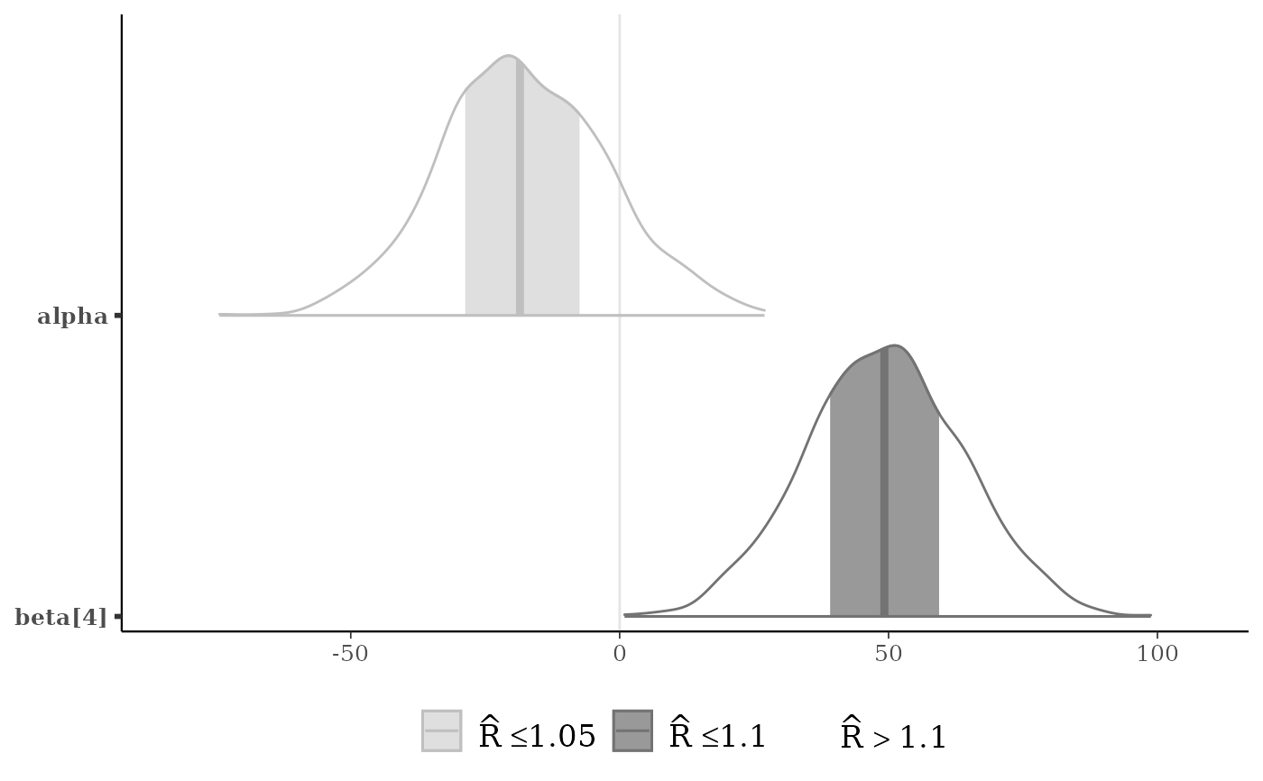
color_scheme_set("gray")
p <- mcmc_areas(x, pars = c("alpha", "beta[4]"), rhat = c(1, 1.1))
p + legend_move("bottom")
# get the dataframe that is used in the plotting functions
mcmc_intervals_data(x)
#> # A tibble: 6 × 9
#> parameter outer_width inner_width point_est ll l m h
#> <fct> <dbl> <dbl> <chr> <dbl> <dbl> <dbl> <dbl>
#> 1 alpha 0.9 0.5 median -42.7 -28.7 -18.5 -7.46
#> 2 sigma 0.9 0.5 median 17.1 17.6 18.0 18.4
#> 3 beta[1] 0.9 0.5 median -0.165 0.136 0.358 0.601
#> 4 beta[2] 0.9 0.5 median -0.722 -0.578 -0.469 -0.362
#> 5 beta[3] 0.9 0.5 median 0.718 0.858 0.950 1.05
#> 6 beta[4] 0.9 0.5 median 24.9 39.1 49.2 59.4
#> # ℹ 1 more variable: hh <dbl>
mcmc_intervals_data(x, rhat = fake_rhat_values)
#> # A tibble: 6 × 12
#> parameter outer_width inner_width point_est ll l m h
#> <fct> <dbl> <dbl> <chr> <dbl> <dbl> <dbl> <dbl>
#> 1 alpha 0.9 0.5 median -42.7 -28.7 -18.5 -7.46
#> 2 sigma 0.9 0.5 median 17.1 17.6 18.0 18.4
#> 3 beta[1] 0.9 0.5 median -0.165 0.136 0.358 0.601
#> 4 beta[2] 0.9 0.5 median -0.722 -0.578 -0.469 -0.362
#> 5 beta[3] 0.9 0.5 median 0.718 0.858 0.950 1.05
#> 6 beta[4] 0.9 0.5 median 24.9 39.1 49.2 59.4
#> # ℹ 4 more variables: hh <dbl>, rhat_value <dbl>, rhat_rating <fct>,
#> # rhat_description <chr>
mcmc_areas_data(x, pars = "alpha")
#> # A tibble: 2,091 × 7
#> parameter interval interval_width x density scaled_density
#> <fct> <chr> <dbl> <dbl> <dbl> <dbl>
#> 1 alpha inner 0.5 -28.7 0.0220 0.865
#> 2 alpha inner 0.5 -28.7 0.0221 0.865
#> 3 alpha inner 0.5 -28.7 0.0221 0.866
#> 4 alpha inner 0.5 -28.7 0.0221 0.866
#> 5 alpha inner 0.5 -28.6 0.0221 0.867
#> 6 alpha inner 0.5 -28.6 0.0221 0.867
#> 7 alpha inner 0.5 -28.6 0.0221 0.868
#> 8 alpha inner 0.5 -28.6 0.0221 0.868
#> 9 alpha inner 0.5 -28.5 0.0222 0.869
#> 10 alpha inner 0.5 -28.5 0.0222 0.870
#> # ℹ 2,081 more rows
#> # ℹ 1 more variable: plotting_density <dbl>
color_scheme_set("gray")
p <- mcmc_areas(x, pars = c("alpha", "beta[4]"), rhat = c(1, 1.1))
p + legend_move("bottom")
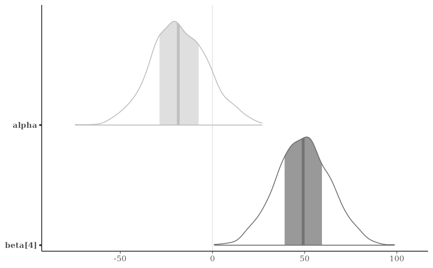
 p + legend_move("none") # or p + legend_none()
 # }
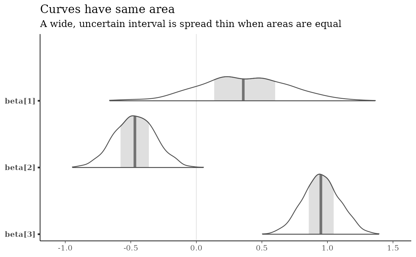
# Different area calculations
b3 <- c("beta[1]", "beta[2]", "beta[3]")
mcmc_areas(x, pars = b3, area_method = "equal area") +
labs(
title = "Curves have same area",
subtitle = "A wide, uncertain interval is spread thin when areas are equal"
)
# }
# Different area calculations
b3 <- c("beta[1]", "beta[2]", "beta[3]")
mcmc_areas(x, pars = b3, area_method = "equal area") +
labs(
title = "Curves have same area",
subtitle = "A wide, uncertain interval is spread thin when areas are equal"
)
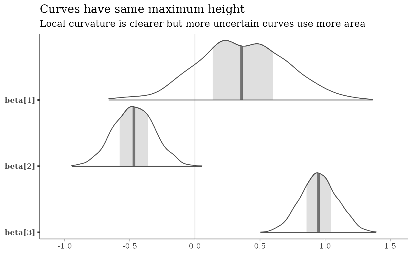
 mcmc_areas(x, pars = b3, area_method = "equal height") +
labs(
title = "Curves have same maximum height",
subtitle = "Local curvature is clearer but more uncertain curves use more area"
)
mcmc_areas(x, pars = b3, area_method = "equal height") +
labs(
title = "Curves have same maximum height",
subtitle = "Local curvature is clearer but more uncertain curves use more area"
)
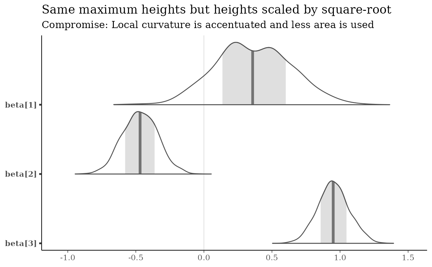
 mcmc_areas(x, pars = b3, area_method = "scaled height") +
labs(
title = "Same maximum heights but heights scaled by square-root",
subtitle = "Compromise: Local curvature is accentuated and less area is used"
)
mcmc_areas(x, pars = b3, area_method = "scaled height") +
labs(
title = "Same maximum heights but heights scaled by square-root",
subtitle = "Compromise: Local curvature is accentuated and less area is used"
)
 # \donttest{
# apply transformations
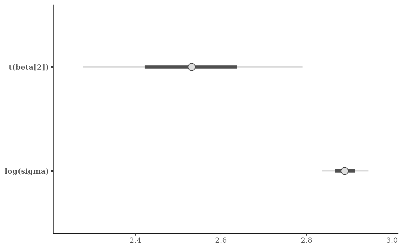
mcmc_intervals(
x,
pars = c("beta[2]", "sigma"),
transformations = list("sigma" = "log", "beta[2]" = function(x) x + 3)
)
# \donttest{
# apply transformations
mcmc_intervals(
x,
pars = c("beta[2]", "sigma"),
transformations = list("sigma" = "log", "beta[2]" = function(x) x + 3)
)
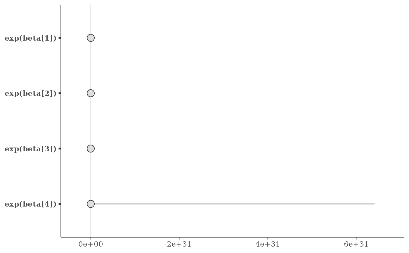
 # apply same transformation to all selected parameters
mcmc_intervals(x, regex_pars = "beta", transformations = "exp")
# apply same transformation to all selected parameters
mcmc_intervals(x, regex_pars = "beta", transformations = "exp")
 # }
# \dontrun{
# example using fitted model from rstanarm package
library(rstanarm)
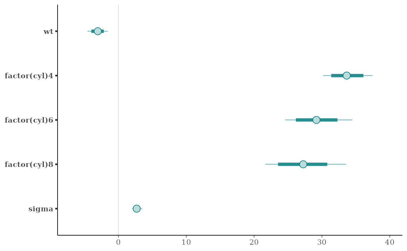
fit <- stan_glm(
mpg ~ 0 + wt + factor(cyl),
data = mtcars,
iter = 500,
refresh = 0
)
#> Warning: Bulk Effective Samples Size (ESS) is too low, indicating posterior means and medians may be unreliable.
#> Running the chains for more iterations may help. See
#> https://mc-stan.org/misc/warnings.html#bulk-ess
#> Warning: Tail Effective Samples Size (ESS) is too low, indicating posterior variances and tail quantiles may be unreliable.
#> Running the chains for more iterations may help. See
#> https://mc-stan.org/misc/warnings.html#tail-ess
x <- as.matrix(fit)
color_scheme_set("teal")
mcmc_intervals(x, point_est = "mean", prob = 0.8, prob_outer = 0.95)
# }
# \dontrun{
# example using fitted model from rstanarm package
library(rstanarm)
fit <- stan_glm(
mpg ~ 0 + wt + factor(cyl),
data = mtcars,
iter = 500,
refresh = 0
)
#> Warning: Bulk Effective Samples Size (ESS) is too low, indicating posterior means and medians may be unreliable.
#> Running the chains for more iterations may help. See
#> https://mc-stan.org/misc/warnings.html#bulk-ess
#> Warning: Tail Effective Samples Size (ESS) is too low, indicating posterior variances and tail quantiles may be unreliable.
#> Running the chains for more iterations may help. See
#> https://mc-stan.org/misc/warnings.html#tail-ess
x <- as.matrix(fit)
color_scheme_set("teal")
mcmc_intervals(x, point_est = "mean", prob = 0.8, prob_outer = 0.95)
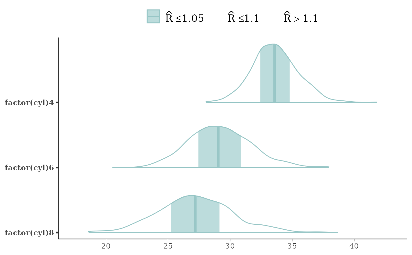
 mcmc_areas(x, regex_pars = "cyl", bw = "SJ",
rhat = rhat(fit, regex_pars = "cyl"))
mcmc_areas(x, regex_pars = "cyl", bw = "SJ",
rhat = rhat(fit, regex_pars = "cyl"))
 # }
# \dontrun{
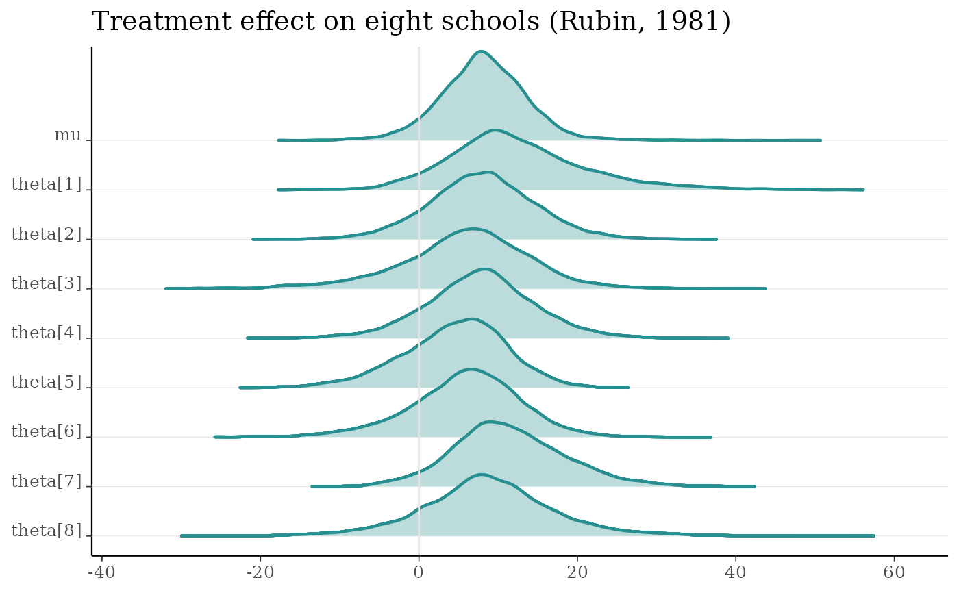
# Example of hierarchically related parameters
# plotted with ridgelines
m <- shinystan::eight_schools@posterior_sample
mcmc_areas_ridges(m, pars = "mu", regex_pars = "theta", border_size = 0.75) +
ggtitle("Treatment effect on eight schools (Rubin, 1981)")
# }
# \dontrun{
# Example of hierarchically related parameters
# plotted with ridgelines
m <- shinystan::eight_schools@posterior_sample
mcmc_areas_ridges(m, pars = "mu", regex_pars = "theta", border_size = 0.75) +
ggtitle("Treatment effect on eight schools (Rubin, 1981)")
 # }
# }