
Stan Development Team
CmdStanR: the R interface to CmdStan.
Details
CmdStanR (cmdstanr package) is an interface to Stan (mc-stan.org) for R users. It provides the necessary objects and functions to compile a Stan program and run Stan's algorithms from R via CmdStan, the command line interface to Stan (mc-stan.org/users/interfaces/cmdstan).
Different ways of interfacing with Stan’s C++
The RStan interface (rstan package)
provides its core functionality through an in-memory interface to Stan
and relies on R packages such as Rcpp to call C++ code from R.
CmdStanR’s core model compilation and inference workflow instead runs
CmdStan in external processes and reads the resulting output files. Only
optional CmdStanR features, such as $expose_functions() and the
additional model methods, use Rcpp to call compiled C++ code
directly from R.
Advantages of RStan
CRAN provides binary versions of RStan for Windows and macOS. RStan-based packages can also include precompiled Stan models in their binary packages, which allows users to run the models without a local C++ toolchain.
CmdStanR-based packages can use
instantiateto compile models once during package installation. Because CRAN’s build machines do not provide CmdStan, packages using this workflow currently need to be installed from source with CmdStan and a C++ toolchain available.Avoids use of R6 classes, which may result in more familiar syntax for many R users.
Advantages of CmdStanR
CmdStan is installed separately from CmdStanR, so users can often update to a new Stan release by updating CmdStan without waiting for a new CmdStanR release.
Running CmdStan in external processes isolates inference from the R process, reducing the risk that a failure during inference terminates the R session.
Potentially lower memory use in the R session. CmdStan writes results to CSV files, and CmdStanR loads draws into R only when requested. This can avoid retaining all output in memory during fitting.
More permissive license. RStan uses the GPL (>= 3) license while the license for CmdStanR is BSD 3-clause, which is a bit more permissive and is the same license used for CmdStan and the Stan C++ source code.
Getting started
CmdStanR requires a working version of CmdStan >=
2.37. If you already have CmdStan installed see cmdstan_model() to get
started, otherwise see install_cmdstan() to install CmdStan. The vignette
Getting started with CmdStanR
demonstrates the basic functionality of the package.
For a list of global options see cmdstanr_global_options.
See also
The CmdStanR website (mc-stan.org/cmdstanr) for online documentation and tutorials.
The Stan and CmdStan documentation:
Stan documentation: mc-stan.org/users/documentation
CmdStan User’s Guide: mc-stan.org/docs/cmdstan-guide
Useful links:
Author
Maintainer: Jonah Gabry jgabry@gmail.com
Authors:
Jonah Gabry jgabry@gmail.com
Rok Češnovar rok.cesnovar@fri.uni-lj.si
Andrew Johnson andrew.johnson@arjohnsonau.com (ORCID)
Steve Bronder
Other contributors:
Ben Bales [contributor]
Mitzi Morris [contributor]
Mikhail Popov [contributor]
Mike Lawrence [contributor]
William Michael Landau will.landau@gmail.com (ORCID) [contributor]
Jacob Socolar [contributor]
Martin Modrák [contributor]
Ven Popov [contributor]
Visruth Srimath Kandali [contributor]
Aki Vehtari [contributor]
Katrina Brock [contributor]
Joss Wright [contributor]
Examples
# \dontrun{
library(cmdstanr)
# If you installed CmdStan with install_cmdstan() the path is already set.
# Otherwise point CmdStanR at your installation with set_cmdstan_path().
cmdstan_path()
#> [1] "/home/runner/.cmdstan/cmdstan-2.40.0"
# Create a CmdStanModel object from a Stan program. This compiles the
# program, or reuses the executable if it's already up to date.
file <- file.path(cmdstan_path(), "examples/bernoulli/bernoulli.stan")
mod <- cmdstan_model(file)
mod$print()
#> data {
#> int<lower=0> N;
#> array[N] int<lower=0, upper=1> y;
#> }
#> parameters {
#> real<lower=0, upper=1> theta;
#> }
#> model {
#> theta ~ beta(1, 1); // uniform prior on interval 0,1
#> y ~ bernoulli(theta);
#> }
# Options for the Stan compiler (stanc_options) and the C++ build
# (cpp_options). dir puts this executable in its own directory instead of
# next to the Stan file, so it doesn't replace the one mod uses. Replace
# tempdir() with a directory you'd keep.
mod_threads <- cmdstan_model(
file,
dir = tempdir(),
stanc_options = list("O1"),
cpp_options = list(stan_threads = TRUE)
)
# What an executable was built from
mod_threads$build_info()
#> Build record: available
#> Reported features:
#> stan_threads: TRUE
#> stan_mpi: FALSE
#> stan_opencl: FALSE
#> stan_no_range_checks: FALSE
#> stan_version: 2.40.0
#> Configuration:
#> cpp_options: STAN_THREADS=true
#> stanc_options: --O1
#> stanc_options_from_make: none
#> include_paths: none
#> Dependencies:
#> stan_file: /home/runner/.cmdstan/cmdstan-2.40.0/examples/bernoulli/bernoulli.stan
#> make_local: /home/runner/.cmdstan/cmdstan-2.40.0/make/local
#> CmdStan 2.40.0 at /home/runner/.cmdstan/cmdstan-2.40.0
# Data is a named list matching the data block
stan_data <- list(N = 10, y = c(0,1,0,0,0,0,0,0,0,1))
# Fit the model with MCMC
fit <- mod$sample(data = stan_data, seed = 123)
#> Running MCMC with 4 sequential chains...
#>
#> Chain 1 Iteration: 1 / 2000 [ 0%] (Warmup)
#> Chain 1 Iteration: 100 / 2000 [ 5%] (Warmup)
#> Chain 1 Iteration: 200 / 2000 [ 10%] (Warmup)
#> Chain 1 Iteration: 300 / 2000 [ 15%] (Warmup)
#> Chain 1 Iteration: 400 / 2000 [ 20%] (Warmup)
#> Chain 1 Iteration: 500 / 2000 [ 25%] (Warmup)
#> Chain 1 Iteration: 600 / 2000 [ 30%] (Warmup)
#> Chain 1 Iteration: 700 / 2000 [ 35%] (Warmup)
#> Chain 1 Iteration: 800 / 2000 [ 40%] (Warmup)
#> Chain 1 Iteration: 900 / 2000 [ 45%] (Warmup)
#> Chain 1 Iteration: 1000 / 2000 [ 50%] (Warmup)
#> Chain 1 Iteration: 1001 / 2000 [ 50%] (Sampling)
#> Chain 1 Iteration: 1100 / 2000 [ 55%] (Sampling)
#> Chain 1 Iteration: 1200 / 2000 [ 60%] (Sampling)
#> Chain 1 Iteration: 1300 / 2000 [ 65%] (Sampling)
#> Chain 1 Iteration: 1400 / 2000 [ 70%] (Sampling)
#> Chain 1 Iteration: 1500 / 2000 [ 75%] (Sampling)
#> Chain 1 Iteration: 1600 / 2000 [ 80%] (Sampling)
#> Chain 1 Iteration: 1700 / 2000 [ 85%] (Sampling)
#> Chain 1 Iteration: 1800 / 2000 [ 90%] (Sampling)
#> Chain 1 Iteration: 1900 / 2000 [ 95%] (Sampling)
#> Chain 1 Iteration: 2000 / 2000 [100%] (Sampling)
#> Chain 1 finished in 0.0 seconds.
#> Chain 2 Iteration: 1 / 2000 [ 0%] (Warmup)
#> Chain 2 Iteration: 100 / 2000 [ 5%] (Warmup)
#> Chain 2 Iteration: 200 / 2000 [ 10%] (Warmup)
#> Chain 2 Iteration: 300 / 2000 [ 15%] (Warmup)
#> Chain 2 Iteration: 400 / 2000 [ 20%] (Warmup)
#> Chain 2 Iteration: 500 / 2000 [ 25%] (Warmup)
#> Chain 2 Iteration: 600 / 2000 [ 30%] (Warmup)
#> Chain 2 Iteration: 700 / 2000 [ 35%] (Warmup)
#> Chain 2 Iteration: 800 / 2000 [ 40%] (Warmup)
#> Chain 2 Iteration: 900 / 2000 [ 45%] (Warmup)
#> Chain 2 Iteration: 1000 / 2000 [ 50%] (Warmup)
#> Chain 2 Iteration: 1001 / 2000 [ 50%] (Sampling)
#> Chain 2 Iteration: 1100 / 2000 [ 55%] (Sampling)
#> Chain 2 Iteration: 1200 / 2000 [ 60%] (Sampling)
#> Chain 2 Iteration: 1300 / 2000 [ 65%] (Sampling)
#> Chain 2 Iteration: 1400 / 2000 [ 70%] (Sampling)
#> Chain 2 Iteration: 1500 / 2000 [ 75%] (Sampling)
#> Chain 2 Iteration: 1600 / 2000 [ 80%] (Sampling)
#> Chain 2 Iteration: 1700 / 2000 [ 85%] (Sampling)
#> Chain 2 Iteration: 1800 / 2000 [ 90%] (Sampling)
#> Chain 2 Iteration: 1900 / 2000 [ 95%] (Sampling)
#> Chain 2 Iteration: 2000 / 2000 [100%] (Sampling)
#> Chain 2 finished in 0.0 seconds.
#> Chain 3 Iteration: 1 / 2000 [ 0%] (Warmup)
#> Chain 3 Iteration: 100 / 2000 [ 5%] (Warmup)
#> Chain 3 Iteration: 200 / 2000 [ 10%] (Warmup)
#> Chain 3 Iteration: 300 / 2000 [ 15%] (Warmup)
#> Chain 3 Iteration: 400 / 2000 [ 20%] (Warmup)
#> Chain 3 Iteration: 500 / 2000 [ 25%] (Warmup)
#> Chain 3 Iteration: 600 / 2000 [ 30%] (Warmup)
#> Chain 3 Iteration: 700 / 2000 [ 35%] (Warmup)
#> Chain 3 Iteration: 800 / 2000 [ 40%] (Warmup)
#> Chain 3 Iteration: 900 / 2000 [ 45%] (Warmup)
#> Chain 3 Iteration: 1000 / 2000 [ 50%] (Warmup)
#> Chain 3 Iteration: 1001 / 2000 [ 50%] (Sampling)
#> Chain 3 Iteration: 1100 / 2000 [ 55%] (Sampling)
#> Chain 3 Iteration: 1200 / 2000 [ 60%] (Sampling)
#> Chain 3 Iteration: 1300 / 2000 [ 65%] (Sampling)
#> Chain 3 Iteration: 1400 / 2000 [ 70%] (Sampling)
#> Chain 3 Iteration: 1500 / 2000 [ 75%] (Sampling)
#> Chain 3 Iteration: 1600 / 2000 [ 80%] (Sampling)
#> Chain 3 Iteration: 1700 / 2000 [ 85%] (Sampling)
#> Chain 3 Iteration: 1800 / 2000 [ 90%] (Sampling)
#> Chain 3 Iteration: 1900 / 2000 [ 95%] (Sampling)
#> Chain 3 Iteration: 2000 / 2000 [100%] (Sampling)
#> Chain 3 finished in 0.0 seconds.
#> Chain 4 Iteration: 1 / 2000 [ 0%] (Warmup)
#> Chain 4 Iteration: 100 / 2000 [ 5%] (Warmup)
#> Chain 4 Iteration: 200 / 2000 [ 10%] (Warmup)
#> Chain 4 Iteration: 300 / 2000 [ 15%] (Warmup)
#> Chain 4 Iteration: 400 / 2000 [ 20%] (Warmup)
#> Chain 4 Iteration: 500 / 2000 [ 25%] (Warmup)
#> Chain 4 Iteration: 600 / 2000 [ 30%] (Warmup)
#> Chain 4 Iteration: 700 / 2000 [ 35%] (Warmup)
#> Chain 4 Iteration: 800 / 2000 [ 40%] (Warmup)
#> Chain 4 Iteration: 900 / 2000 [ 45%] (Warmup)
#> Chain 4 Iteration: 1000 / 2000 [ 50%] (Warmup)
#> Chain 4 Iteration: 1001 / 2000 [ 50%] (Sampling)
#> Chain 4 Iteration: 1100 / 2000 [ 55%] (Sampling)
#> Chain 4 Iteration: 1200 / 2000 [ 60%] (Sampling)
#> Chain 4 Iteration: 1300 / 2000 [ 65%] (Sampling)
#> Chain 4 Iteration: 1400 / 2000 [ 70%] (Sampling)
#> Chain 4 Iteration: 1500 / 2000 [ 75%] (Sampling)
#> Chain 4 Iteration: 1600 / 2000 [ 80%] (Sampling)
#> Chain 4 Iteration: 1700 / 2000 [ 85%] (Sampling)
#> Chain 4 Iteration: 1800 / 2000 [ 90%] (Sampling)
#> Chain 4 Iteration: 1900 / 2000 [ 95%] (Sampling)
#> Chain 4 Iteration: 2000 / 2000 [100%] (Sampling)
#> Chain 4 finished in 0.0 seconds.
#>
#> All 4 chains finished successfully.
#> Mean chain execution time: 0.0 seconds.
#> Total execution time: 0.5 seconds.
#>
fit$summary()
#> # A tibble: 2 × 10
#> variable mean median sd mad q5 q95 rhat ess_bulk ess_tail
#> <chr> <dbl> <dbl> <dbl> <dbl> <dbl> <dbl> <dbl> <dbl> <dbl>
#> 1 lp__ -7.30 -7.01 0.805 0.345 -8.82 -6.75 1.00 1834. 2187.
#> 2 theta 0.257 0.243 0.124 0.126 0.0792 0.486 1.00 1165. 1581.
fit$diagnostic_summary()
#> $num_divergent
#> [1] 0 0 0 0
#>
#> $num_max_treedepth
#> [1] 0 0 0 0
#>
#> $ebfmi
#> [1] 1.114870 1.030279 1.053383 1.077471
#>
# Posterior draws, here as a posterior::draws_df
fit$draws(format = "df")
#> # A draws_df: 1000 iterations, 4 chains, and 2 variables
#> lp__ theta
#> 1 -7.0 0.17
#> 2 -7.9 0.46
#> 3 -7.4 0.41
#> 4 -6.7 0.25
#> 5 -6.9 0.18
#> 6 -6.9 0.33
#> 7 -7.2 0.15
#> 8 -6.8 0.29
#> 9 -6.8 0.24
#> 10 -6.8 0.24
#> # ... with 3990 more draws
#> # ... hidden reserved variables {'.chain', '.iteration', '.draw'}
# Plot with bayesplot
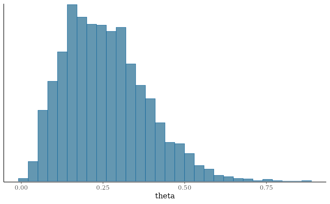
bayesplot::mcmc_hist(fit$draws("theta"))
#> `stat_bin()` using `bins = 30`. Pick better value `binwidth`.
 # }
# }