PPC errors

Various plots of predictive errors y - yrep. See the Details and Plot Descriptions sections, below.

Usage

ppc_error_hist(
  y,
  yrep,
  ...,
  facet_args = list(),
  binwidth = NULL,
  bins = NULL,
  breaks = NULL,
  freq = TRUE
)

ppc_error_hist_grouped(
  y,
  yrep,
  group,
  ...,
  facet_args = list(),
  binwidth = NULL,
  bins = NULL,
  breaks = NULL,
  freq = TRUE
)

ppc_error_scatter(y, yrep, ..., facet_args = list(), size = 2.5, alpha = 0.8)

ppc_error_scatter_avg(
  y,
  yrep,
  x = NULL,
  ...,
  stat = "mean",
  size = 2.5,
  alpha = 0.8
)

ppc_error_scatter_avg_grouped(
  y,
  yrep,
  group,
  ...,
  stat = "mean",
  facet_args = list(),
  size = 2.5,
  alpha = 0.8
)

ppc_error_scatter_avg_vs_x(
  y,
  yrep,
  x,
  ...,
  stat = "mean",
  size = 2.5,
  alpha = 0.8
)

ppc_error_binned(
  y,
  yrep,
  x = NULL,
  ...,
  facet_args = list(),
  bins = NULL,
  size = 1,
  alpha = 0.25
)

ppc_error_data(y, yrep, group = NULL)

Arguments

y: A vector of observations. See Details.
yrep: An S by N matrix of draws from the posterior (or prior) predictive distribution, or a posterior::draws object. The number of rows, S, is the size of the posterior (or prior) sample used to generate yrep. The number of columns, N is the number of predicted observations (length(y)). The columns of yrep should be in the same order as the data points in y for the plots to make sense. See the Details and Plot Descriptions sections for additional advice specific to particular plots.
...: Currently unused.
facet_args: A named list of arguments (other than facets) passed to ggplot2::facet_wrap() or ggplot2::facet_grid() to control faceting. Note: if scales is not included in facet_args then bayesplot may use scales="free" as the default (depending on the plot) instead of the ggplot2 default of scales="fixed".
binwidth: Passed to ggplot2::geom_histogram(), ggplot2::geom_area(), and ggdist::stat_dots() to override the default binwidth.
bins: For ppc_error_binned(), the number of bins to use (approximately).
breaks: Passed to ggplot2::geom_histogram() as an alternative to binwidth.
freq: For histograms and frequency polygons, freq=TRUE (the default) puts count on the y-axis. Setting freq=FALSE puts density on the y-axis. (For many plots the y-axis text is off by default. To view the count or density labels on the y-axis see the yaxis_text() convenience function.)
group: A grouping variable of the same length as y. Will be coerced to factor if not already a factor. Each value in group is interpreted as the group level pertaining to the corresponding observation.
size, alpha: For scatterplots, arguments passed to ggplot2::geom_point() to control the appearance of the points. For the binned error plot, arguments controlling the size of the outline and opacity of the shaded region indicating the 2-SE bounds.
x: A numeric vector the same length as y to use as the x-axis variable.
stat: A function or a string naming a function for computing the posterior average. In both cases, the function should take a vector input and return a scalar statistic. The function name is displayed in the axis-label. Defaults to "mean".

Value

The plotting functions return a ggplot object that can be further customized using the ggplot2 package. The functions with suffix _data() return the data that would have been drawn by the plotting function.

Details

All of these functions (aside from the *_scatter_avg functions) compute and plot predictive errors for each row of the matrix yrep, so it is usually a good idea for yrep to contain only a small number of draws (rows). See Examples, below.

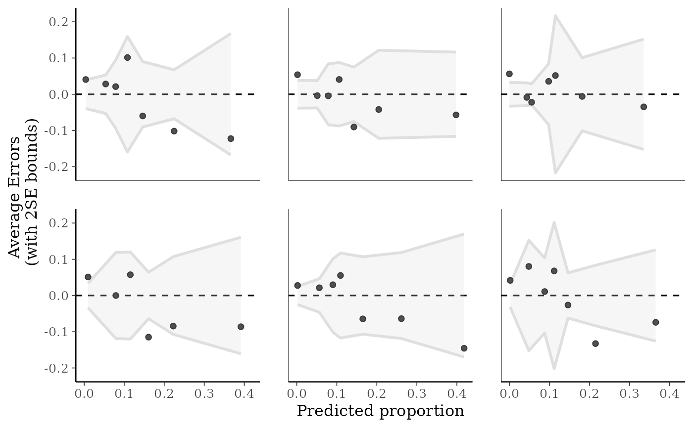
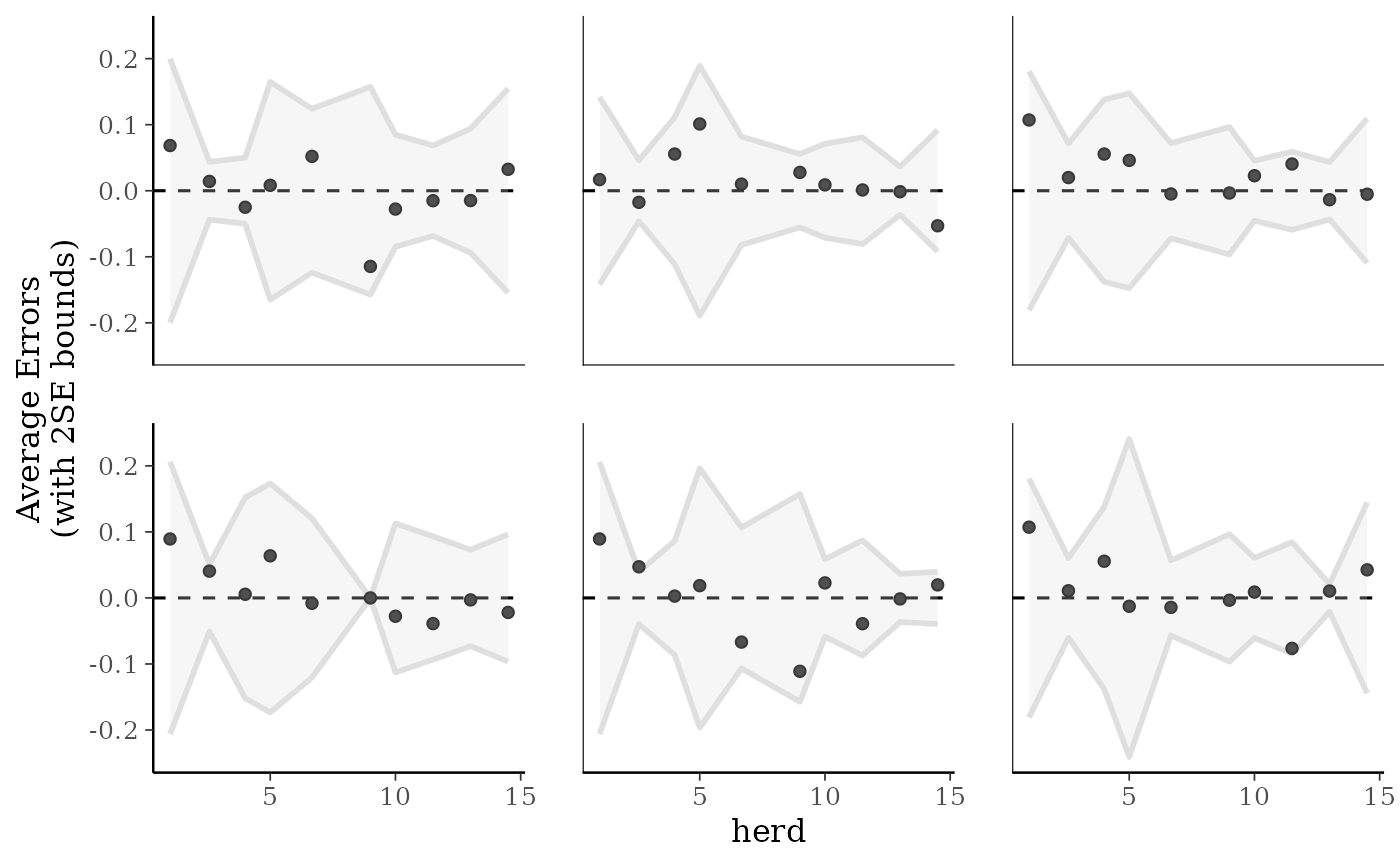
For binomial and Bernoulli data the ppc_error_binned() function can be used to generate binned error plots. Bernoulli data can be input as a vector of 0s and 1s, whereas for binomial data y and yrep should contain "success" proportions (not counts). See the Examples section, below.

Plot descriptions

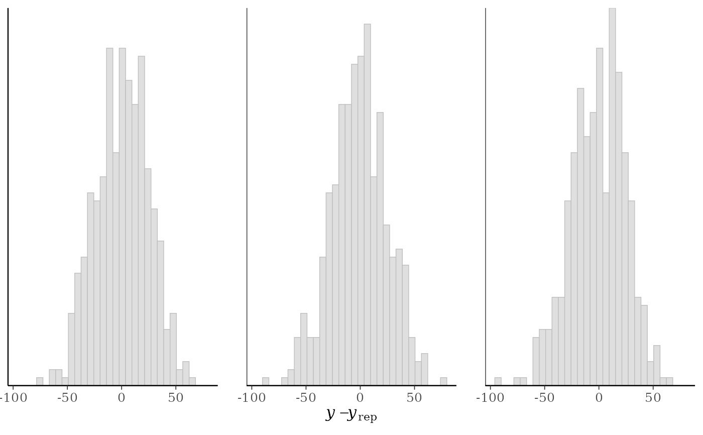
ppc_error_hist()

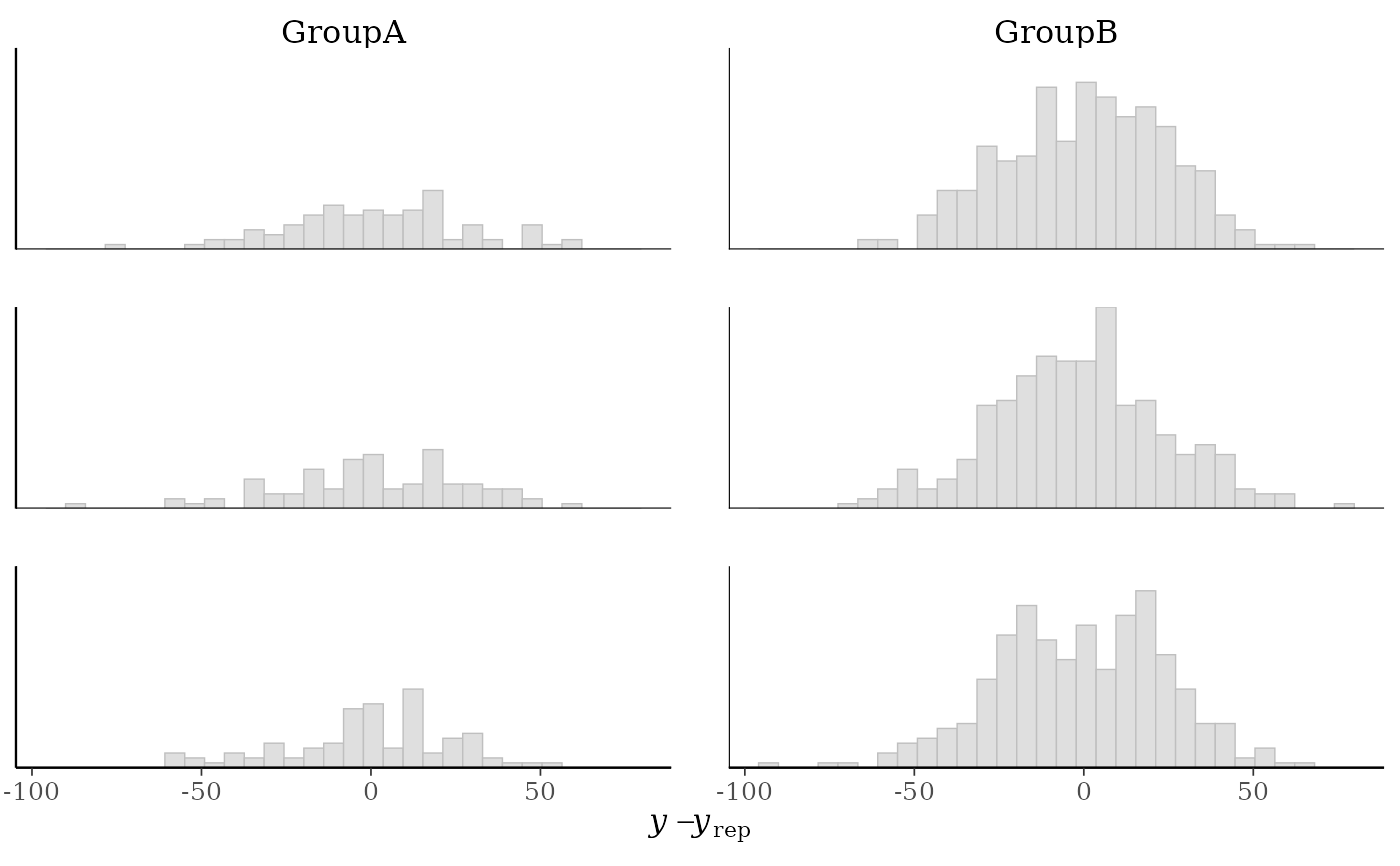
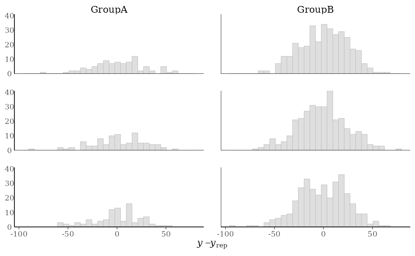
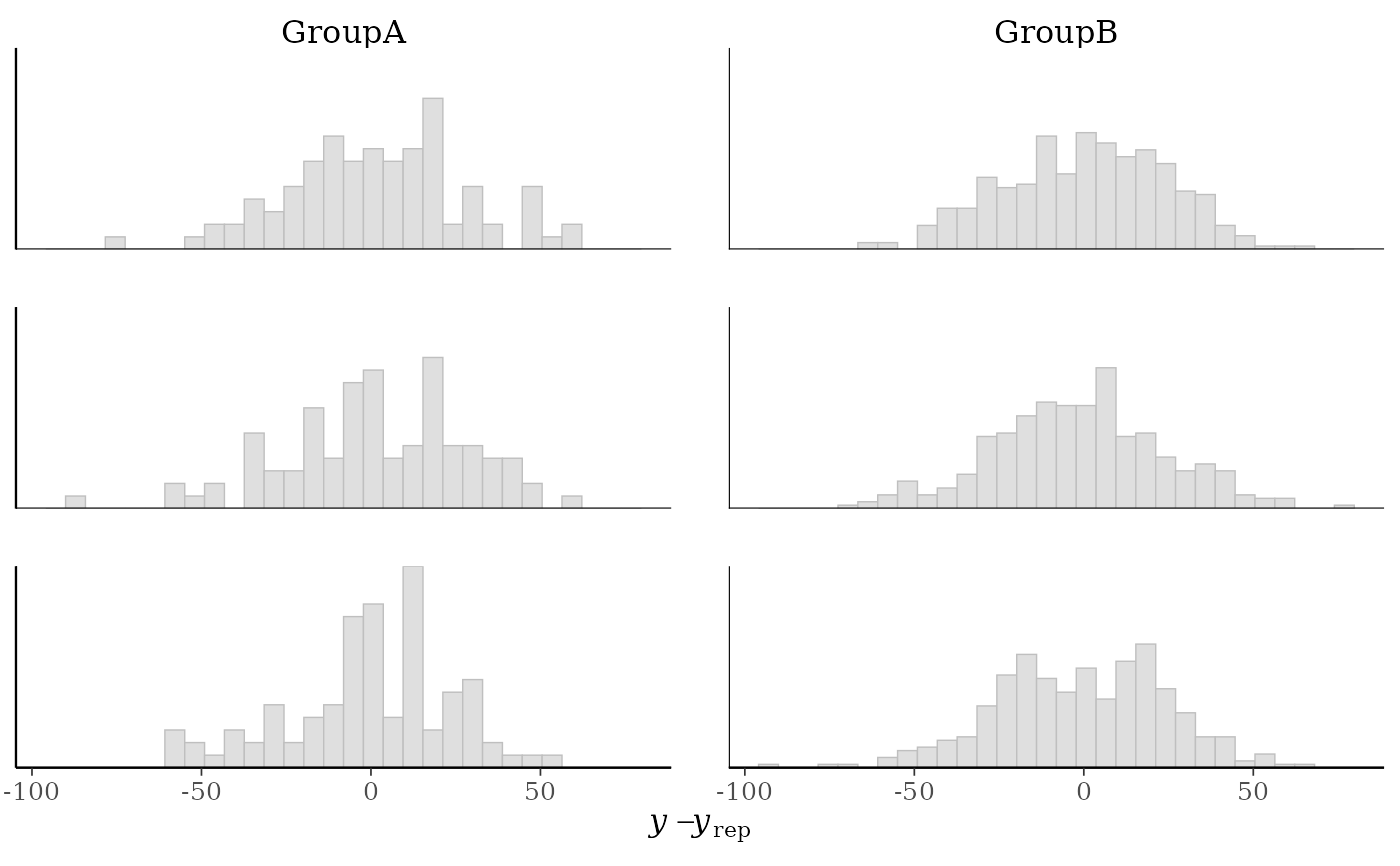
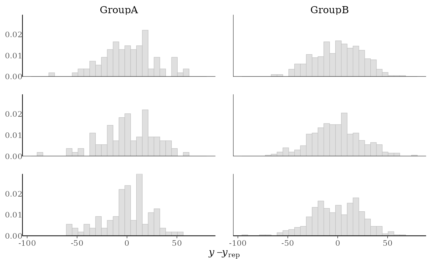
A separate histogram is plotted for the predictive errors computed from y and each dataset (row) in yrep. For this plot yrep should have only a small number of rows.

ppc_error_hist_grouped()

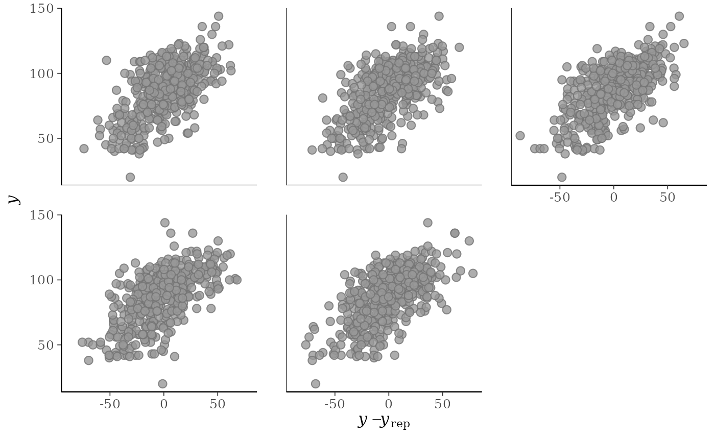
Like ppc_error_hist(), except errors are computed within levels of a grouping variable. The number of histograms is therefore equal to the product of the number of rows in yrep and the number of groups (unique values of group).

ppc_error_scatter()

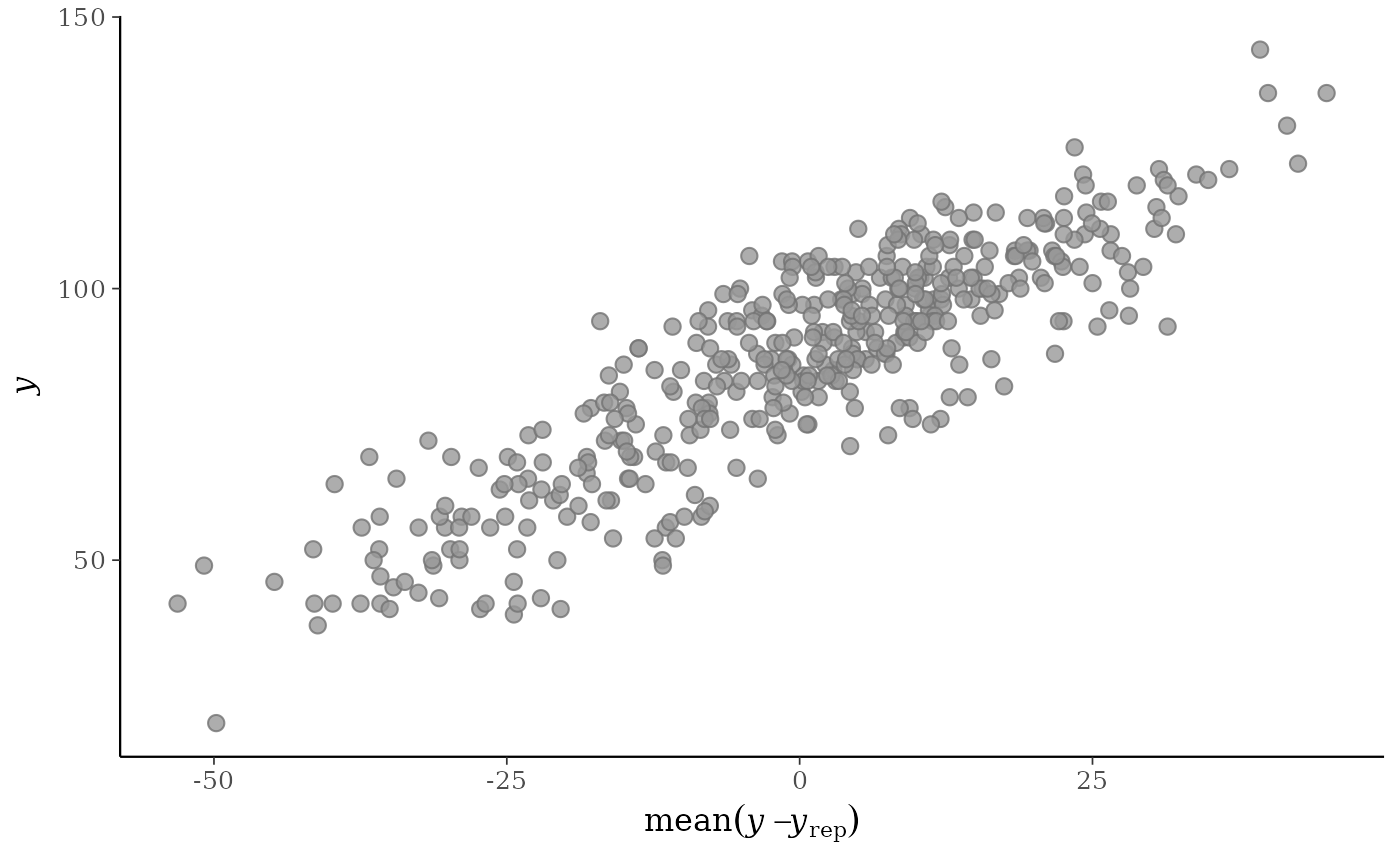
A separate scatterplot is displayed for y vs. the predictive errors computed from y and each dataset (row) in yrep. For this plot yrep should have only a small number of rows.

ppc_error_scatter_avg()

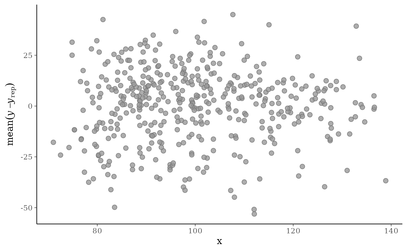
A single scatterplot of y vs. the average of the errors computed from y and each dataset (row) in yrep. For each individual data point y[n] the average error is the average of the errors for y[n] computed over the the draws from the posterior predictive distribution.

When the optional x argument is provided, the average error is plotted on the y-axis and the predictor variable x is plotted on the x-axis.

ppc_error_scatter_avg_vs_x()

Deprecated. Use ppc_error_scatter_avg(x = x) instead.

ppc_error_binned()

Intended for use with binomial data. A separate binned error plot (similar to arm::binnedplot()) is generated for each dataset (row) in yrep. For this plot y and yrep should contain proportions rather than counts, and yrep should have only a small number of rows.

ppc_error_data()

Data-preparation back end for the ppc_error_*() family of plotting functions. Users can call ppc_error_data() directly to obtain the data frame of predictive errors (y - yrep) and create custom error visualizations with ggplot2.

References

Gelman, A., Carlin, J. B., Stern, H. S., Dunson, D. B., Vehtari, A., and Rubin, D. B. (2013). Bayesian Data Analysis. Chapman & Hall/CRC Press, London, third edition. (Ch. 6)

Examples

y <- example_y_data()
yrep <- example_yrep_draws()
ppc_error_hist(y, yrep[1:3, ])
#> `stat_bin()` using `bins = 30`. Pick better value `binwidth`.


# errors within groups
group <- example_group_data()
(p1 <- ppc_error_hist_grouped(y, yrep[1:3, ], group))
#> `stat_bin()` using `bins = 30`. Pick better value `binwidth`.

p1 + yaxis_text() # defaults to showing counts on y-axis
#> `stat_bin()` using `bins = 30`. Pick better value `binwidth`.

# \donttest{
table(group) # more obs in GroupB, can set freq=FALSE to show density on y-axis
#> group
#> GroupA GroupB 
#>     93    341 
(p2 <- ppc_error_hist_grouped(y, yrep[1:3, ], group, freq = FALSE))
#> `stat_bin()` using `bins = 30`. Pick better value `binwidth`.

p2 + yaxis_text()
#> `stat_bin()` using `bins = 30`. Pick better value `binwidth`.

# }

# scatterplots
ppc_error_scatter(y, yrep[10:14, ])

ppc_error_scatter_avg(y, yrep)


x <- example_x_data()
ppc_error_scatter_avg(y, yrep, x)


# \dontrun{
# binned error plot with binomial model from rstanarm
library(rstanarm)
example("example_model", package = "rstanarm")
#> 
#> exmpl_> if (.Platform$OS.type != "windows" || .Platform$r_arch != "i386") {
#> exmpl_+ example_model <- 
#> exmpl_+   stan_glmer(cbind(incidence, size - incidence) ~ size + period + (1|herd),
#> exmpl_+              data = lme4::cbpp, family = binomial, QR = TRUE,
#> exmpl_+              # this next line is only to keep the example small in size!
#> exmpl_+              chains = 2, cores = 1, seed = 12345, iter = 1000, refresh = 0)
#> exmpl_+ example_model
#> exmpl_+ }
#> stan_glmer
#>  family:       binomial [logit]
#>  formula:      cbind(incidence, size - incidence) ~ size + period + (1 | herd)
#>  observations: 56
#> ------
#>             Median MAD_SD
#> (Intercept) -1.5    0.6  
#> size         0.0    0.0  
#> period2     -1.0    0.3  
#> period3     -1.1    0.4  
#> period4     -1.6    0.5  
#> 
#> Error terms:
#>  Groups Name        Std.Dev.
#>  herd   (Intercept) 0.76    
#> Num. levels: herd 15 
#> 
#> ------
#> * For help interpreting the printed output see ?print.stanreg
#> * For info on the priors used see ?prior_summary.stanreg
formula(example_model)
#> cbind(incidence, size - incidence) ~ size + period + (1 | herd)

# get observed proportion of "successes"
y <- example_model$y  # matrix of "success" and "failure" counts
trials <- rowSums(y)
y_prop <- y[, 1] / trials  # proportions

# get predicted success proportions
yrep <- posterior_predict(example_model)
yrep_prop <- sweep(yrep, 2, trials, "/")

ppc_error_binned(y_prop, yrep_prop[1:6, ])


# plotting against a covariate on x-axis
herd <- as.numeric(example_model$data$herd)
ppc_error_binned(y_prop, yrep_prop[1:6, ], x = herd)

# }