Simulation Based Calibration

Here is a Stan program for a beta-binomial model

data {
  int<lower = 1> N;
  real<lower = 0> a;
  real<lower = 0> b;
}
transformed data { // these adhere to the conventions above
  real pi_ = beta_rng(a, b);
  int y = binomial_rng(N, pi_);
}
parameters {
  real<lower = 0, upper = 1> pi;
}
model {
  target += beta_lpdf(pi | a, b);
  target += binomial_lpmf(y | N, pi);
}
generated quantities { // these adhere to the conventions above
  int y_ = y;
  vector[1] pars_;
  int ranks_[1] = {pi > pi_};
  vector[N] log_lik;
  pars_[1] = pi_;
  for (n in 1:y) log_lik[n] = bernoulli_lpmf(1 | pi);
  for (n in (y + 1):N) log_lik[n] = bernoulli_lpmf(0 | pi);
}

Notice that it adheres to the following conventions:

Realizations of the unknown parameters are drawn in the transformed data block are postfixed with an underscore, such as pi_. These are considered the “true” parameters being estimated by the corresponding symbol declared in the parameters block, which have the same names except for the trailing underscore, such as pi.
The realizations of the unknown parameters are then conditioned on when drawing from the prior predictive distribution in transformed data block, which in this case is int y = binomial_rng(N, pi_);. To avoid confusion, y does not have a training underscore.
The realizations of the unknown parameters are copied into a vector in the generated quantities block named pars_
The realizations from the prior predictive distribution are copied into an object (of the same type) in the generated quantities block named `y_. This is optional.
The generated quantities block contains an integer array named ranks_ whose only values are zero or one, depending on whether the realization of a parameter from the posterior distribution exceeds the corresponding “true” realization, which in this case is ranks_[1] = {pi > pi_};. These are not actually “ranks” but can be used afterwards to reconstruct (thinned) ranks.
The generated quantities block contains a vector named log_lik whose values are the contribution to the log-likelihood by each observation. In this case, the “observations” are the implicit successes and failures that are aggregated into a binomial likelihood. This is optional but facilitates calculating the Pareto k shape parameter estimates that indicate whether the posterior distribution is sensitive to particular observations.

Assuming the above is compile to a code stanmodel named beta_binomial, we can then call the sbc function

output <- sbc(beta_binomial, data = list(N = 10, a = 1, b = 1), M = 500, refresh = 0)

At which point, we can then call

print(output)

## 0 chains had divergent transitions after warmup

plot(output, bins = 10) # it is best to specify the bins argument yourself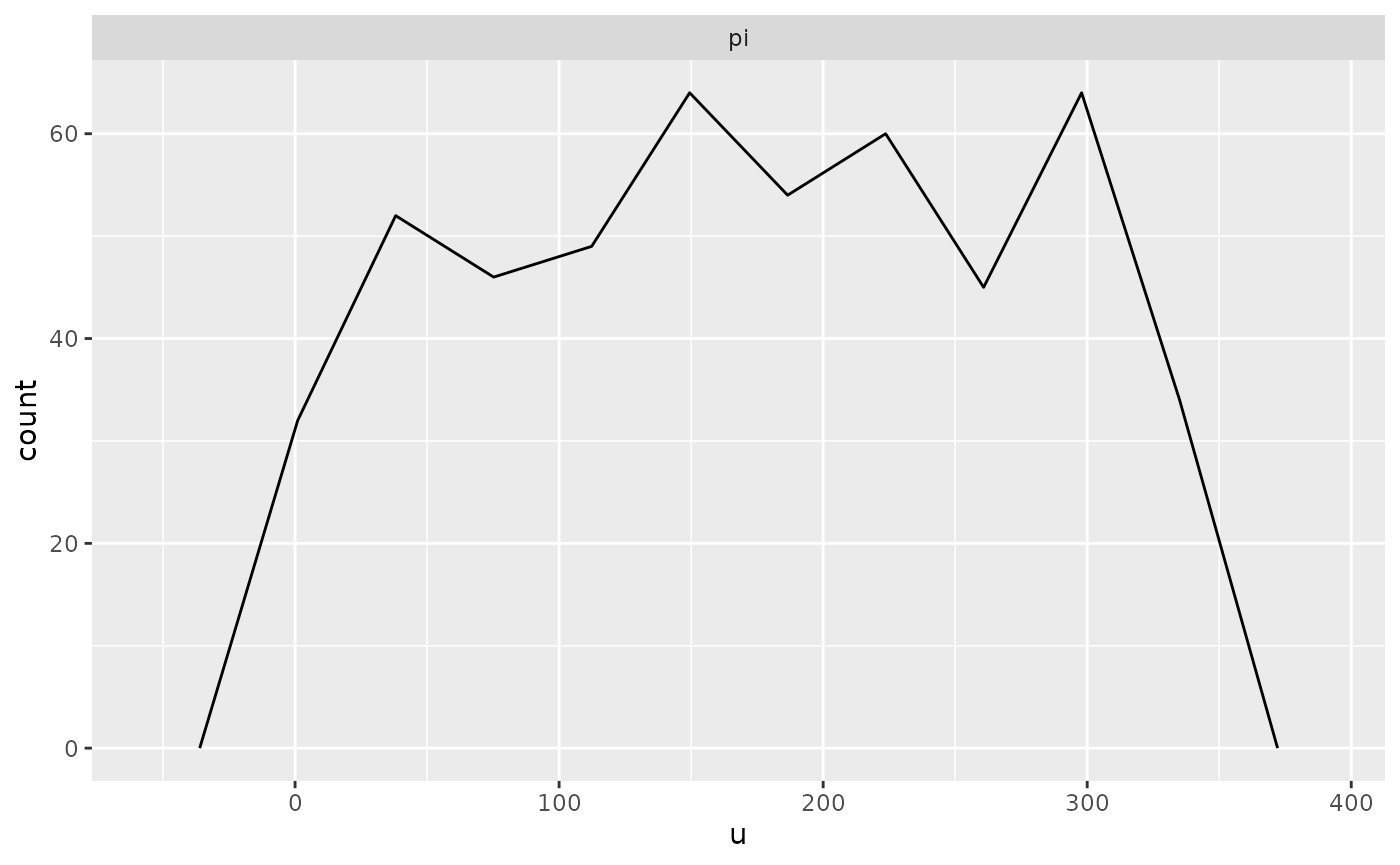

References

Talts, S., Betancourt, M., Simpson, D., Vehtari, A., and Gelman, A. (2018). Validating Bayesian Inference Algorithms with Simulation-Based Calibration. arXiv preprint arXiv:1804.06788

Stan Development Team

2023-09-08

References