Create a new CmdStanModel object from a file containing a Stan program
or from an existing Stan executable. The CmdStanModel object stores the
path to a Stan program and compiled executable (once created), and provides
methods for fitting the model using Stan's algorithms.
See the compile and ... arguments for control over whether and how
compilation happens.
cmdstan_model(stan_file = NULL, exe_file = NULL, compile = TRUE, ...)Arguments
- stan_file
(string) The path to a
.stanfile containing a Stan program. The helper functionwrite_stan_file()is provided for cases when it is more convenient to specify the Stan program as a string. Ifstan_fileis not specified thenexe_filemust be specified.- exe_file
(string) The path to an existing Stan model executable. Can be provided instead of or in addition to
stan_file(ifstan_fileis omitted someCmdStanModelmethods like$code()and$print()will not work). This argument can only be used with CmdStan 2.27+.- compile
(logical) Do compilation? The default is
TRUE. IfFALSEcompilation can be done later via the$compile()method.- ...
Optionally, additional arguments to pass to the
$compile()method ifcompile=TRUE. These options include specifying the directory for saving the executable, turning on pedantic mode, specifying include paths, configuring C++ options, and more. See$compile()for details.
Value
A CmdStanModel object.
See also
install_cmdstan(), $compile(),
$check_syntax()
The CmdStanR website (mc-stan.org/cmdstanr) for online documentation and tutorials.
The Stan and CmdStan documentation:
Stan documentation: mc-stan.org/users/documentation
CmdStan User’s Guide: mc-stan.org/docs/cmdstan-guide
Examples
# \dontrun{
library(cmdstanr)
library(posterior)
library(bayesplot)
color_scheme_set("brightblue")
# Set path to CmdStan
# (Note: if you installed CmdStan via install_cmdstan() with default settings
# then setting the path is unnecessary but the default below should still work.
# Otherwise use the `path` argument to specify the location of your
# CmdStan installation.)
set_cmdstan_path(path = NULL)
#> CmdStan path set to: /Users/jgabry/.cmdstan/cmdstan-2.36.0
# Create a CmdStanModel object from a Stan program,
# here using the example model that comes with CmdStan
file <- file.path(cmdstan_path(), "examples/bernoulli/bernoulli.stan")
mod <- cmdstan_model(file)
mod$print()
#> data {
#> int<lower=0> N;
#> array[N] int<lower=0, upper=1> y;
#> }
#> parameters {
#> real<lower=0, upper=1> theta;
#> }
#> model {
#> theta ~ beta(1, 1); // uniform prior on interval 0,1
#> y ~ bernoulli(theta);
#> }
# Print with line numbers. This can be set globally using the
# `cmdstanr_print_line_numbers` option.
mod$print(line_numbers = TRUE)
#> 1: data {
#> 2: int<lower=0> N;
#> 3: array[N] int<lower=0, upper=1> y;
#> 4: }
#> 5: parameters {
#> 6: real<lower=0, upper=1> theta;
#> 7: }
#> 8: model {
#> 9: theta ~ beta(1, 1); // uniform prior on interval 0,1
#> 10: y ~ bernoulli(theta);
#> 11: }
# Data as a named list (like RStan)
stan_data <- list(N = 10, y = c(0,1,0,0,0,0,0,0,0,1))
# Run MCMC using the 'sample' method
fit_mcmc <- mod$sample(
data = stan_data,
seed = 123,
chains = 2,
parallel_chains = 2
)
#> Running MCMC with 2 parallel chains...
#>
#> Chain 1 Iteration: 1 / 2000 [ 0%] (Warmup)
#> Chain 1 Iteration: 100 / 2000 [ 5%] (Warmup)
#> Chain 1 Iteration: 200 / 2000 [ 10%] (Warmup)
#> Chain 1 Iteration: 300 / 2000 [ 15%] (Warmup)
#> Chain 1 Iteration: 400 / 2000 [ 20%] (Warmup)
#> Chain 1 Iteration: 500 / 2000 [ 25%] (Warmup)
#> Chain 1 Iteration: 600 / 2000 [ 30%] (Warmup)
#> Chain 1 Iteration: 700 / 2000 [ 35%] (Warmup)
#> Chain 1 Iteration: 800 / 2000 [ 40%] (Warmup)
#> Chain 1 Iteration: 900 / 2000 [ 45%] (Warmup)
#> Chain 1 Iteration: 1000 / 2000 [ 50%] (Warmup)
#> Chain 1 Iteration: 1001 / 2000 [ 50%] (Sampling)
#> Chain 1 Iteration: 1100 / 2000 [ 55%] (Sampling)
#> Chain 1 Iteration: 1200 / 2000 [ 60%] (Sampling)
#> Chain 1 Iteration: 1300 / 2000 [ 65%] (Sampling)
#> Chain 1 Iteration: 1400 / 2000 [ 70%] (Sampling)
#> Chain 1 Iteration: 1500 / 2000 [ 75%] (Sampling)
#> Chain 1 Iteration: 1600 / 2000 [ 80%] (Sampling)
#> Chain 1 Iteration: 1700 / 2000 [ 85%] (Sampling)
#> Chain 1 Iteration: 1800 / 2000 [ 90%] (Sampling)
#> Chain 1 Iteration: 1900 / 2000 [ 95%] (Sampling)
#> Chain 1 Iteration: 2000 / 2000 [100%] (Sampling)
#> Chain 2 Iteration: 1 / 2000 [ 0%] (Warmup)
#> Chain 2 Iteration: 100 / 2000 [ 5%] (Warmup)
#> Chain 2 Iteration: 200 / 2000 [ 10%] (Warmup)
#> Chain 2 Iteration: 300 / 2000 [ 15%] (Warmup)
#> Chain 2 Iteration: 400 / 2000 [ 20%] (Warmup)
#> Chain 2 Iteration: 500 / 2000 [ 25%] (Warmup)
#> Chain 2 Iteration: 600 / 2000 [ 30%] (Warmup)
#> Chain 2 Iteration: 700 / 2000 [ 35%] (Warmup)
#> Chain 2 Iteration: 800 / 2000 [ 40%] (Warmup)
#> Chain 2 Iteration: 900 / 2000 [ 45%] (Warmup)
#> Chain 2 Iteration: 1000 / 2000 [ 50%] (Warmup)
#> Chain 2 Iteration: 1001 / 2000 [ 50%] (Sampling)
#> Chain 2 Iteration: 1100 / 2000 [ 55%] (Sampling)
#> Chain 2 Iteration: 1200 / 2000 [ 60%] (Sampling)
#> Chain 2 Iteration: 1300 / 2000 [ 65%] (Sampling)
#> Chain 2 Iteration: 1400 / 2000 [ 70%] (Sampling)
#> Chain 2 Iteration: 1500 / 2000 [ 75%] (Sampling)
#> Chain 2 Iteration: 1600 / 2000 [ 80%] (Sampling)
#> Chain 2 Iteration: 1700 / 2000 [ 85%] (Sampling)
#> Chain 2 Iteration: 1800 / 2000 [ 90%] (Sampling)
#> Chain 2 Iteration: 1900 / 2000 [ 95%] (Sampling)
#> Chain 2 Iteration: 2000 / 2000 [100%] (Sampling)
#> Chain 1 finished in 0.0 seconds.
#> Chain 2 finished in 0.0 seconds.
#>
#> Both chains finished successfully.
#> Mean chain execution time: 0.0 seconds.
#> Total execution time: 0.2 seconds.
#>
# Use 'posterior' package for summaries
fit_mcmc$summary()
#> # A tibble: 2 × 10
#> variable mean median sd mad q5 q95 rhat ess_bulk ess_tail
#> <chr> <dbl> <dbl> <dbl> <dbl> <dbl> <dbl> <dbl> <dbl> <dbl>
#> 1 lp__ -7.35 -7.01 0.882 0.353 -9.14 -6.75 1.00 724. 896.
#> 2 theta 0.254 0.239 0.129 0.126 0.0737 0.488 1.00 532. 657.
# Check sampling diagnostics
fit_mcmc$diagnostic_summary()
#> $num_divergent
#> [1] 0 0
#>
#> $num_max_treedepth
#> [1] 0 0
#>
#> $ebfmi
#> [1] 1.1148479 0.7568734
#>
# Get posterior draws
draws <- fit_mcmc$draws()
print(draws)
#> # A draws_array: 1000 iterations, 2 chains, and 2 variables
#> , , variable = lp__
#>
#> chain
#> iteration 1 2
#> 1 -7.0 -8.1
#> 2 -7.9 -7.9
#> 3 -7.4 -7.0
#> 4 -6.7 -6.8
#> 5 -6.9 -6.8
#>
#> , , variable = theta
#>
#> chain
#> iteration 1 2
#> 1 0.17 0.088
#> 2 0.46 0.097
#> 3 0.41 0.167
#> 4 0.25 0.292
#> 5 0.18 0.238
#>
#> # ... with 995 more iterations
# Convert to data frame using posterior::as_draws_df
as_draws_df(draws)
#> # A draws_df: 1000 iterations, 2 chains, and 2 variables
#> lp__ theta
#> 1 -7.0 0.17
#> 2 -7.9 0.46
#> 3 -7.4 0.41
#> 4 -6.7 0.25
#> 5 -6.9 0.18
#> 6 -6.9 0.33
#> 7 -7.2 0.15
#> 8 -6.8 0.29
#> 9 -6.8 0.24
#> 10 -6.8 0.24
#> # ... with 1990 more draws
#> # ... hidden reserved variables {'.chain', '.iteration', '.draw'}
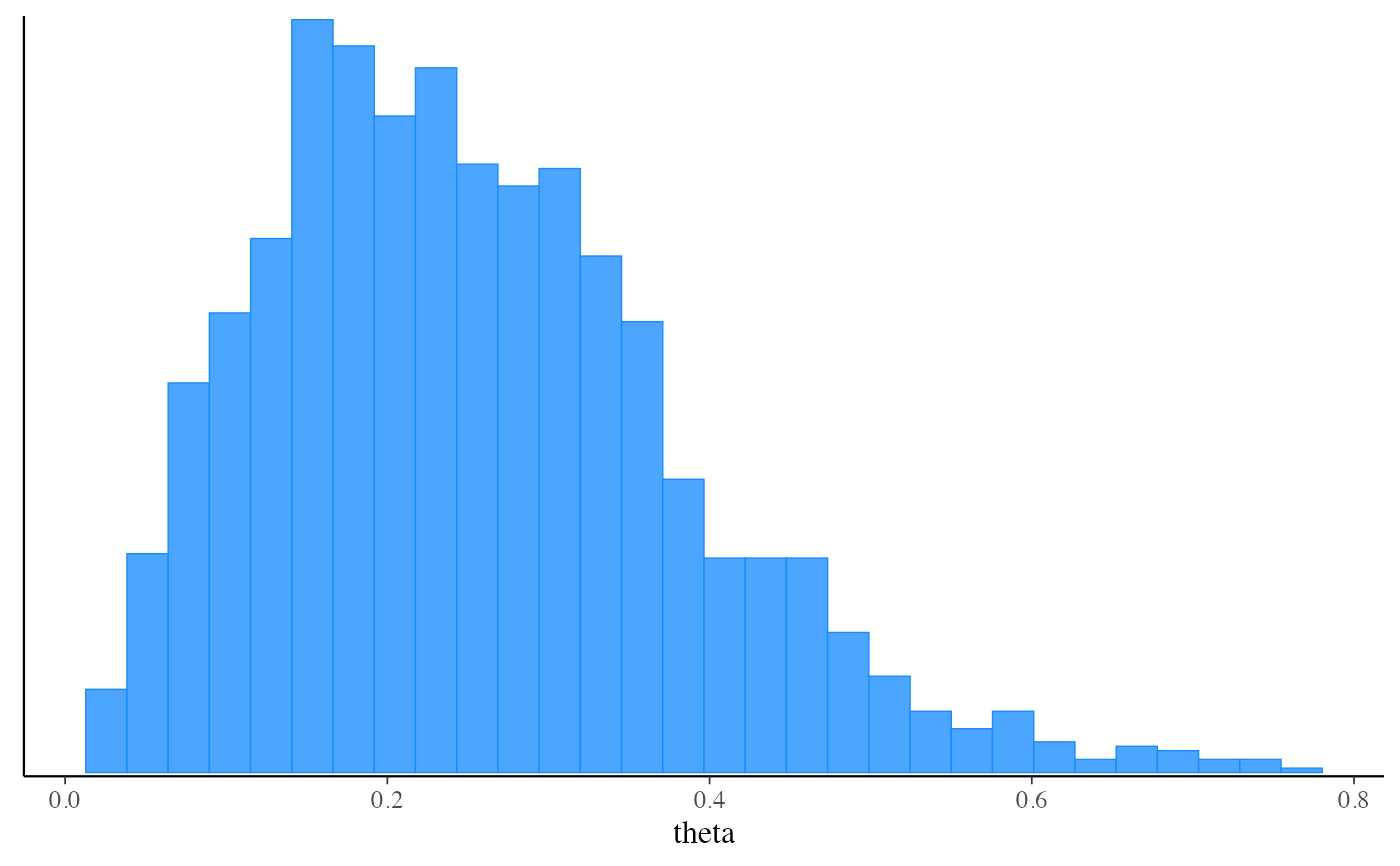
# Plot posterior using bayesplot (ggplot2)
mcmc_hist(fit_mcmc$draws("theta"))
#> `stat_bin()` using `bins = 30`. Pick better value with `binwidth`.
 # Run 'optimize' method to get a point estimate (default is Stan's LBFGS algorithm)
# and also demonstrate specifying data as a path to a file instead of a list
my_data_file <- file.path(cmdstan_path(), "examples/bernoulli/bernoulli.data.json")
fit_optim <- mod$optimize(data = my_data_file, seed = 123)
#> Initial log joint probability = -16.144
#> Iter log prob ||dx|| ||grad|| alpha alpha0 # evals Notes
#> 6 -5.00402 0.000246518 8.73164e-07 1 1 9
#> Optimization terminated normally:
#> Convergence detected: relative gradient magnitude is below tolerance
#> Finished in 0.1 seconds.
fit_optim$summary()
#> # A tibble: 2 × 2
#> variable estimate
#> <chr> <dbl>
#> 1 lp__ -5.00
#> 2 theta 0.2
# Run 'optimize' again with 'jacobian=TRUE' and then draw from Laplace approximation
# to the posterior
fit_optim <- mod$optimize(data = my_data_file, jacobian = TRUE)
#> Initial log joint probability = -7.19041
#> Iter log prob ||dx|| ||grad|| alpha alpha0 # evals Notes
#> 5 -6.74802 0.000219546 2.02164e-07 1 1 8
#> Optimization terminated normally:
#> Convergence detected: relative gradient magnitude is below tolerance
#> Finished in 0.1 seconds.
fit_laplace <- mod$laplace(data = my_data_file, mode = fit_optim, draws = 2000)
#> Calculating Hessian
#> Calculating inverse of Cholesky factor
#> Generating draws
#> iteration: 0
#> iteration: 100
#> iteration: 200
#> iteration: 300
#> iteration: 400
#> iteration: 500
#> iteration: 600
#> iteration: 700
#> iteration: 800
#> iteration: 900
#> iteration: 1000
#> iteration: 1100
#> iteration: 1200
#> iteration: 1300
#> iteration: 1400
#> iteration: 1500
#> iteration: 1600
#> iteration: 1700
#> iteration: 1800
#> iteration: 1900
#> Finished in 0.1 seconds.
fit_laplace$summary()
#> # A tibble: 3 × 7
#> variable mean median sd mad q5 q95
#> <chr> <dbl> <dbl> <dbl> <dbl> <dbl> <dbl>
#> 1 lp__ -7.23 -6.98 0.662 0.312 -8.57 -6.75
#> 2 lp_approx__ -0.490 -0.230 0.676 0.315 -1.92 -0.00147
#> 3 theta 0.269 0.251 0.121 0.123 0.101 0.490
# Run 'variational' method to use ADVI to approximate posterior
fit_vb <- mod$variational(data = stan_data, seed = 123)
#> ------------------------------------------------------------
#> EXPERIMENTAL ALGORITHM:
#> This procedure has not been thoroughly tested and may be unstable
#> or buggy. The interface is subject to change.
#> ------------------------------------------------------------
#> Gradient evaluation took 9e-06 seconds
#> 1000 transitions using 10 leapfrog steps per transition would take 0.09 seconds.
#> Adjust your expectations accordingly!
#> Begin eta adaptation.
#> Iteration: 1 / 250 [ 0%] (Adaptation)
#> Iteration: 50 / 250 [ 20%] (Adaptation)
#> Iteration: 100 / 250 [ 40%] (Adaptation)
#> Iteration: 150 / 250 [ 60%] (Adaptation)
#> Iteration: 200 / 250 [ 80%] (Adaptation)
#> Success! Found best value [eta = 1] earlier than expected.
#> Begin stochastic gradient ascent.
#> iter ELBO delta_ELBO_mean delta_ELBO_med notes
#> 100 -6.164 1.000 1.000
#> 200 -6.225 0.505 1.000
#> 300 -6.186 0.339 0.010 MEDIAN ELBO CONVERGED
#> Drawing a sample of size 1000 from the approximate posterior...
#> COMPLETED.
#> Finished in 0.1 seconds.
fit_vb$summary()
#> # A tibble: 3 × 7
#> variable mean median sd mad q5 q95
#> <chr> <dbl> <dbl> <dbl> <dbl> <dbl> <dbl>
#> 1 lp__ -7.14 -6.93 0.528 0.247 -8.21 -6.75
#> 2 lp_approx__ -0.520 -0.244 0.740 0.326 -1.90 -0.00227
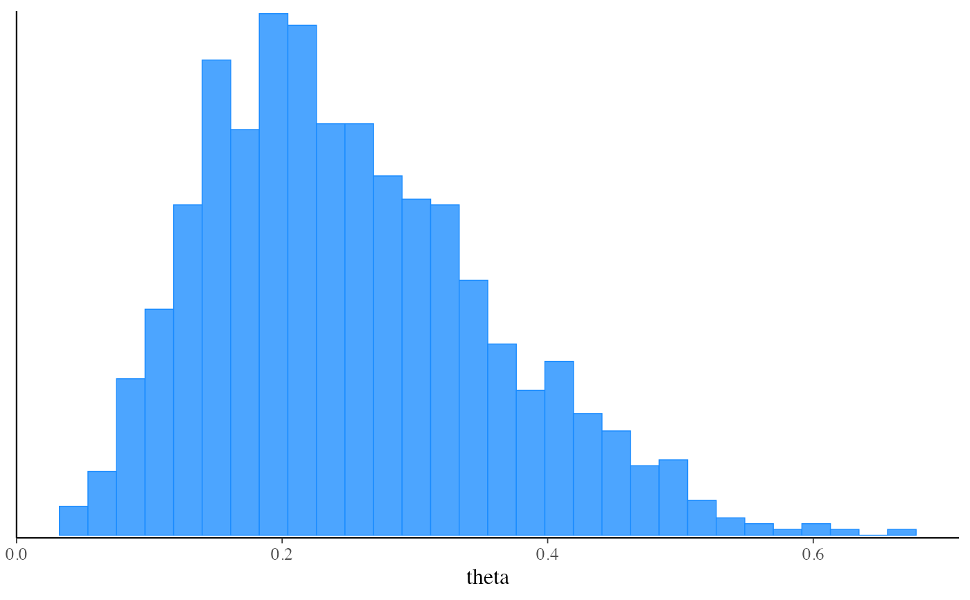
#> 3 theta 0.251 0.236 0.107 0.108 0.100 0.446
mcmc_hist(fit_vb$draws("theta"))
#> `stat_bin()` using `bins = 30`. Pick better value with `binwidth`.
# Run 'optimize' method to get a point estimate (default is Stan's LBFGS algorithm)
# and also demonstrate specifying data as a path to a file instead of a list
my_data_file <- file.path(cmdstan_path(), "examples/bernoulli/bernoulli.data.json")
fit_optim <- mod$optimize(data = my_data_file, seed = 123)
#> Initial log joint probability = -16.144
#> Iter log prob ||dx|| ||grad|| alpha alpha0 # evals Notes
#> 6 -5.00402 0.000246518 8.73164e-07 1 1 9
#> Optimization terminated normally:
#> Convergence detected: relative gradient magnitude is below tolerance
#> Finished in 0.1 seconds.
fit_optim$summary()
#> # A tibble: 2 × 2
#> variable estimate
#> <chr> <dbl>
#> 1 lp__ -5.00
#> 2 theta 0.2
# Run 'optimize' again with 'jacobian=TRUE' and then draw from Laplace approximation
# to the posterior
fit_optim <- mod$optimize(data = my_data_file, jacobian = TRUE)
#> Initial log joint probability = -7.19041
#> Iter log prob ||dx|| ||grad|| alpha alpha0 # evals Notes
#> 5 -6.74802 0.000219546 2.02164e-07 1 1 8
#> Optimization terminated normally:
#> Convergence detected: relative gradient magnitude is below tolerance
#> Finished in 0.1 seconds.
fit_laplace <- mod$laplace(data = my_data_file, mode = fit_optim, draws = 2000)
#> Calculating Hessian
#> Calculating inverse of Cholesky factor
#> Generating draws
#> iteration: 0
#> iteration: 100
#> iteration: 200
#> iteration: 300
#> iteration: 400
#> iteration: 500
#> iteration: 600
#> iteration: 700
#> iteration: 800
#> iteration: 900
#> iteration: 1000
#> iteration: 1100
#> iteration: 1200
#> iteration: 1300
#> iteration: 1400
#> iteration: 1500
#> iteration: 1600
#> iteration: 1700
#> iteration: 1800
#> iteration: 1900
#> Finished in 0.1 seconds.
fit_laplace$summary()
#> # A tibble: 3 × 7
#> variable mean median sd mad q5 q95
#> <chr> <dbl> <dbl> <dbl> <dbl> <dbl> <dbl>
#> 1 lp__ -7.23 -6.98 0.662 0.312 -8.57 -6.75
#> 2 lp_approx__ -0.490 -0.230 0.676 0.315 -1.92 -0.00147
#> 3 theta 0.269 0.251 0.121 0.123 0.101 0.490
# Run 'variational' method to use ADVI to approximate posterior
fit_vb <- mod$variational(data = stan_data, seed = 123)
#> ------------------------------------------------------------
#> EXPERIMENTAL ALGORITHM:
#> This procedure has not been thoroughly tested and may be unstable
#> or buggy. The interface is subject to change.
#> ------------------------------------------------------------
#> Gradient evaluation took 9e-06 seconds
#> 1000 transitions using 10 leapfrog steps per transition would take 0.09 seconds.
#> Adjust your expectations accordingly!
#> Begin eta adaptation.
#> Iteration: 1 / 250 [ 0%] (Adaptation)
#> Iteration: 50 / 250 [ 20%] (Adaptation)
#> Iteration: 100 / 250 [ 40%] (Adaptation)
#> Iteration: 150 / 250 [ 60%] (Adaptation)
#> Iteration: 200 / 250 [ 80%] (Adaptation)
#> Success! Found best value [eta = 1] earlier than expected.
#> Begin stochastic gradient ascent.
#> iter ELBO delta_ELBO_mean delta_ELBO_med notes
#> 100 -6.164 1.000 1.000
#> 200 -6.225 0.505 1.000
#> 300 -6.186 0.339 0.010 MEDIAN ELBO CONVERGED
#> Drawing a sample of size 1000 from the approximate posterior...
#> COMPLETED.
#> Finished in 0.1 seconds.
fit_vb$summary()
#> # A tibble: 3 × 7
#> variable mean median sd mad q5 q95
#> <chr> <dbl> <dbl> <dbl> <dbl> <dbl> <dbl>
#> 1 lp__ -7.14 -6.93 0.528 0.247 -8.21 -6.75
#> 2 lp_approx__ -0.520 -0.244 0.740 0.326 -1.90 -0.00227
#> 3 theta 0.251 0.236 0.107 0.108 0.100 0.446
mcmc_hist(fit_vb$draws("theta"))
#> `stat_bin()` using `bins = 30`. Pick better value with `binwidth`.
 # Run 'pathfinder' method, a new alternative to the variational method
fit_pf <- mod$pathfinder(data = stan_data, seed = 123)
#> Path [1] :Initial log joint density = -18.273334
#> Path [1] : Iter log prob ||dx|| ||grad|| alpha alpha0 # evals ELBO Best ELBO Notes
#> 5 -6.748e+00 7.082e-04 1.432e-05 1.000e+00 1.000e+00 126 -6.145e+00 -6.145e+00
#> Path [1] :Best Iter: [5] ELBO (-6.145070) evaluations: (126)
#> Path [2] :Initial log joint density = -19.192715
#> Path [2] : Iter log prob ||dx|| ||grad|| alpha alpha0 # evals ELBO Best ELBO Notes
#> 5 -6.748e+00 2.015e-04 2.228e-06 1.000e+00 1.000e+00 126 -6.223e+00 -6.223e+00
#> Path [2] :Best Iter: [2] ELBO (-6.170358) evaluations: (126)
#> Path [3] :Initial log joint density = -6.774820
#> Path [3] : Iter log prob ||dx|| ||grad|| alpha alpha0 # evals ELBO Best ELBO Notes
#> 4 -6.748e+00 1.137e-04 2.596e-07 1.000e+00 1.000e+00 101 -6.178e+00 -6.178e+00
#> Path [3] :Best Iter: [4] ELBO (-6.177909) evaluations: (101)
#> Path [4] :Initial log joint density = -7.949193
#> Path [4] : Iter log prob ||dx|| ||grad|| alpha alpha0 # evals ELBO Best ELBO Notes
#> 5 -6.748e+00 2.145e-04 1.301e-06 1.000e+00 1.000e+00 126 -6.197e+00 -6.197e+00
#> Path [4] :Best Iter: [5] ELBO (-6.197118) evaluations: (126)
#> Total log probability function evaluations:4379
#> Finished in 0.1 seconds.
fit_pf$summary()
#> # A tibble: 3 × 7
#> variable mean median sd mad q5 q95
#> <chr> <dbl> <dbl> <dbl> <dbl> <dbl> <dbl>
#> 1 lp_approx__ -1.07 -0.727 0.945 0.311 -2.91 -0.450
#> 2 lp__ -7.25 -6.97 0.753 0.308 -8.78 -6.75
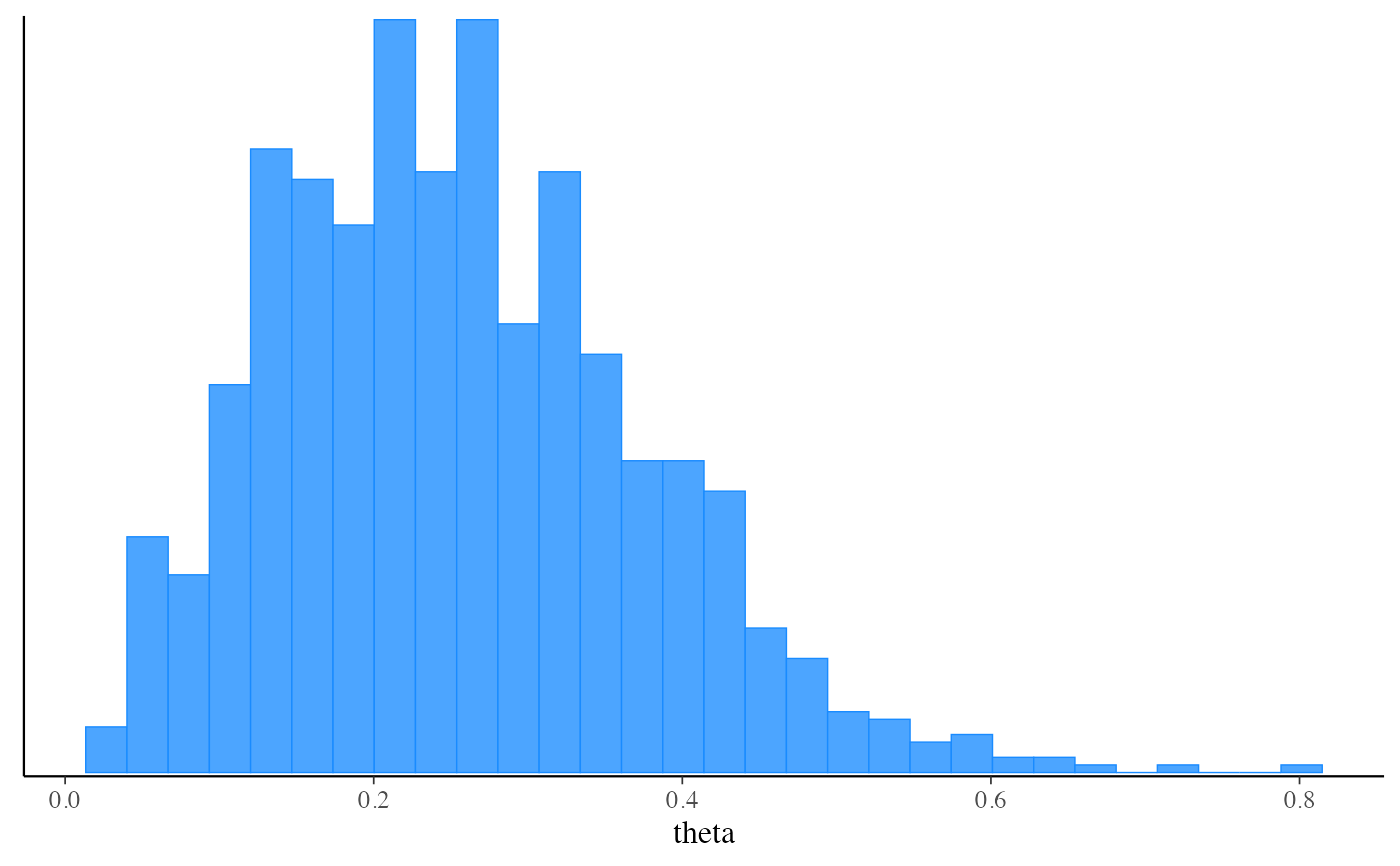
#> 3 theta 0.256 0.245 0.119 0.123 0.0824 0.462
mcmc_hist(fit_pf$draws("theta"))
#> `stat_bin()` using `bins = 30`. Pick better value with `binwidth`.
# Run 'pathfinder' method, a new alternative to the variational method
fit_pf <- mod$pathfinder(data = stan_data, seed = 123)
#> Path [1] :Initial log joint density = -18.273334
#> Path [1] : Iter log prob ||dx|| ||grad|| alpha alpha0 # evals ELBO Best ELBO Notes
#> 5 -6.748e+00 7.082e-04 1.432e-05 1.000e+00 1.000e+00 126 -6.145e+00 -6.145e+00
#> Path [1] :Best Iter: [5] ELBO (-6.145070) evaluations: (126)
#> Path [2] :Initial log joint density = -19.192715
#> Path [2] : Iter log prob ||dx|| ||grad|| alpha alpha0 # evals ELBO Best ELBO Notes
#> 5 -6.748e+00 2.015e-04 2.228e-06 1.000e+00 1.000e+00 126 -6.223e+00 -6.223e+00
#> Path [2] :Best Iter: [2] ELBO (-6.170358) evaluations: (126)
#> Path [3] :Initial log joint density = -6.774820
#> Path [3] : Iter log prob ||dx|| ||grad|| alpha alpha0 # evals ELBO Best ELBO Notes
#> 4 -6.748e+00 1.137e-04 2.596e-07 1.000e+00 1.000e+00 101 -6.178e+00 -6.178e+00
#> Path [3] :Best Iter: [4] ELBO (-6.177909) evaluations: (101)
#> Path [4] :Initial log joint density = -7.949193
#> Path [4] : Iter log prob ||dx|| ||grad|| alpha alpha0 # evals ELBO Best ELBO Notes
#> 5 -6.748e+00 2.145e-04 1.301e-06 1.000e+00 1.000e+00 126 -6.197e+00 -6.197e+00
#> Path [4] :Best Iter: [5] ELBO (-6.197118) evaluations: (126)
#> Total log probability function evaluations:4379
#> Finished in 0.1 seconds.
fit_pf$summary()
#> # A tibble: 3 × 7
#> variable mean median sd mad q5 q95
#> <chr> <dbl> <dbl> <dbl> <dbl> <dbl> <dbl>
#> 1 lp_approx__ -1.07 -0.727 0.945 0.311 -2.91 -0.450
#> 2 lp__ -7.25 -6.97 0.753 0.308 -8.78 -6.75
#> 3 theta 0.256 0.245 0.119 0.123 0.0824 0.462
mcmc_hist(fit_pf$draws("theta"))
#> `stat_bin()` using `bins = 30`. Pick better value with `binwidth`.
 # Run 'pathfinder' again with more paths, fewer draws per path,
# better covariance approximation, and fewer LBFGSs iterations
fit_pf <- mod$pathfinder(data = stan_data, num_paths=10, single_path_draws=40,
history_size=50, max_lbfgs_iters=100)
#> Warning: Number of PSIS draws is larger than the total number of draws returned by the single Pathfinders. This is likely unintentional and leads to re-sampling from the same draws.
#> Path [1] :Initial log joint density = -19.520956
#> Path [1] : Iter log prob ||dx|| ||grad|| alpha alpha0 # evals ELBO Best ELBO Notes
#> 4 -6.748e+00 1.226e-02 1.762e-04 1.000e+00 1.000e+00 101 -6.253e+00 -6.253e+00
#> Path [1] :Best Iter: [2] ELBO (-6.195755) evaluations: (101)
#> Path [2] :Initial log joint density = -7.254863
#> Path [2] : Iter log prob ||dx|| ||grad|| alpha alpha0 # evals ELBO Best ELBO Notes
#> 5 -6.748e+00 3.135e-04 3.796e-07 1.000e+00 1.000e+00 126 -6.215e+00 -6.215e+00
#> Path [2] :Best Iter: [4] ELBO (-6.093719) evaluations: (126)
#> Path [3] :Initial log joint density = -9.357651
#> Path [3] : Iter log prob ||dx|| ||grad|| alpha alpha0 # evals ELBO Best ELBO Notes
#> 5 -6.748e+00 4.272e-04 4.080e-06 1.000e+00 1.000e+00 126 -6.228e+00 -6.228e+00
#> Path [3] :Best Iter: [3] ELBO (-6.197602) evaluations: (126)
#> Path [4] :Initial log joint density = -15.654513
#> Path [4] : Iter log prob ||dx|| ||grad|| alpha alpha0 # evals ELBO Best ELBO Notes
#> 5 -6.748e+00 1.955e-03 5.901e-05 1.000e+00 1.000e+00 126 -6.224e+00 -6.224e+00
#> Path [4] :Best Iter: [5] ELBO (-6.224416) evaluations: (126)
#> Path [5] :Initial log joint density = -6.893187
#> Path [5] : Iter log prob ||dx|| ||grad|| alpha alpha0 # evals ELBO Best ELBO Notes
#> 4 -6.748e+00 1.780e-04 2.911e-05 9.344e-01 9.344e-01 101 -6.239e+00 -6.239e+00
#> Path [5] :Best Iter: [3] ELBO (-6.215896) evaluations: (101)
#> Path [6] :Initial log joint density = -10.329090
#> Path [6] : Iter log prob ||dx|| ||grad|| alpha alpha0 # evals ELBO Best ELBO Notes
#> 5 -6.748e+00 7.385e-04 9.583e-06 1.000e+00 1.000e+00 126 -6.222e+00 -6.222e+00
#> Path [6] :Best Iter: [3] ELBO (-6.212303) evaluations: (126)
#> Path [7] :Initial log joint density = -15.872224
#> Path [7] : Iter log prob ||dx|| ||grad|| alpha alpha0 # evals ELBO Best ELBO Notes
#> 5 -6.748e+00 1.903e-03 5.733e-05 1.000e+00 1.000e+00 126 -6.254e+00 -6.254e+00
#> Path [7] :Best Iter: [4] ELBO (-6.195869) evaluations: (126)
#> Path [8] :Initial log joint density = -10.958418
#> Path [8] : Iter log prob ||dx|| ||grad|| alpha alpha0 # evals ELBO Best ELBO Notes
#> 5 -6.748e+00 9.246e-04 1.360e-05 1.000e+00 1.000e+00 126 -6.214e+00 -6.214e+00
#> Path [8] :Best Iter: [2] ELBO (-6.186854) evaluations: (126)
#> Path [9] :Initial log joint density = -12.861849
#> Path [9] : Iter log prob ||dx|| ||grad|| alpha alpha0 # evals ELBO Best ELBO Notes
#> 5 -6.748e+00 1.621e-03 3.641e-05 1.000e+00 1.000e+00 126 -6.213e+00 -6.213e+00
#> Path [9] :Best Iter: [5] ELBO (-6.213458) evaluations: (126)
#> Path [10] :Initial log joint density = -16.360860
#> Path [10] : Iter log prob ||dx|| ||grad|| alpha alpha0 # evals ELBO Best ELBO Notes
#> 5 -6.748e+00 1.745e-03 5.153e-05 1.000e+00 1.000e+00 126 -6.169e+00 -6.169e+00
#> Path [10] :Best Iter: [5] ELBO (-6.169190) evaluations: (126)
#> Total log probability function evaluations:1360
#> Finished in 0.1 seconds.
# Specifying initial values as a function
fit_mcmc_w_init_fun <- mod$sample(
data = stan_data,
seed = 123,
chains = 2,
refresh = 0,
init = function() list(theta = runif(1))
)
#> Running MCMC with 2 sequential chains...
#>
#> Chain 1 finished in 0.0 seconds.
#> Chain 2 finished in 0.0 seconds.
#>
#> Both chains finished successfully.
#> Mean chain execution time: 0.0 seconds.
#> Total execution time: 0.3 seconds.
#>
fit_mcmc_w_init_fun_2 <- mod$sample(
data = stan_data,
seed = 123,
chains = 2,
refresh = 0,
init = function(chain_id) {
# silly but demonstrates optional use of chain_id
list(theta = 1 / (chain_id + 1))
}
)
#> Running MCMC with 2 sequential chains...
#>
#> Chain 1 finished in 0.0 seconds.
#> Chain 2 finished in 0.0 seconds.
#>
#> Both chains finished successfully.
#> Mean chain execution time: 0.0 seconds.
#> Total execution time: 0.3 seconds.
#>
fit_mcmc_w_init_fun_2$init()
#> [[1]]
#> [[1]]$theta
#> [1] 0.5
#>
#>
#> [[2]]
#> [[2]]$theta
#> [1] 0.3333333
#>
#>
# Specifying initial values as a list of lists
fit_mcmc_w_init_list <- mod$sample(
data = stan_data,
seed = 123,
chains = 2,
refresh = 0,
init = list(
list(theta = 0.75), # chain 1
list(theta = 0.25) # chain 2
)
)
#> Running MCMC with 2 sequential chains...
#>
#> Chain 1 finished in 0.0 seconds.
#> Chain 2 finished in 0.0 seconds.
#>
#> Both chains finished successfully.
#> Mean chain execution time: 0.0 seconds.
#> Total execution time: 0.3 seconds.
#>
fit_optim_w_init_list <- mod$optimize(
data = stan_data,
seed = 123,
init = list(
list(theta = 0.75)
)
)
#> Initial log joint probability = -11.6657
#> Iter log prob ||dx|| ||grad|| alpha alpha0 # evals Notes
#> 6 -5.00402 0.000237915 9.55309e-07 1 1 9
#> Optimization terminated normally:
#> Convergence detected: relative gradient magnitude is below tolerance
#> Finished in 0.1 seconds.
fit_optim_w_init_list$init()
#> [[1]]
#> [[1]]$theta
#> [1] 0.75
#>
#>
# }
# Run 'pathfinder' again with more paths, fewer draws per path,
# better covariance approximation, and fewer LBFGSs iterations
fit_pf <- mod$pathfinder(data = stan_data, num_paths=10, single_path_draws=40,
history_size=50, max_lbfgs_iters=100)
#> Warning: Number of PSIS draws is larger than the total number of draws returned by the single Pathfinders. This is likely unintentional and leads to re-sampling from the same draws.
#> Path [1] :Initial log joint density = -19.520956
#> Path [1] : Iter log prob ||dx|| ||grad|| alpha alpha0 # evals ELBO Best ELBO Notes
#> 4 -6.748e+00 1.226e-02 1.762e-04 1.000e+00 1.000e+00 101 -6.253e+00 -6.253e+00
#> Path [1] :Best Iter: [2] ELBO (-6.195755) evaluations: (101)
#> Path [2] :Initial log joint density = -7.254863
#> Path [2] : Iter log prob ||dx|| ||grad|| alpha alpha0 # evals ELBO Best ELBO Notes
#> 5 -6.748e+00 3.135e-04 3.796e-07 1.000e+00 1.000e+00 126 -6.215e+00 -6.215e+00
#> Path [2] :Best Iter: [4] ELBO (-6.093719) evaluations: (126)
#> Path [3] :Initial log joint density = -9.357651
#> Path [3] : Iter log prob ||dx|| ||grad|| alpha alpha0 # evals ELBO Best ELBO Notes
#> 5 -6.748e+00 4.272e-04 4.080e-06 1.000e+00 1.000e+00 126 -6.228e+00 -6.228e+00
#> Path [3] :Best Iter: [3] ELBO (-6.197602) evaluations: (126)
#> Path [4] :Initial log joint density = -15.654513
#> Path [4] : Iter log prob ||dx|| ||grad|| alpha alpha0 # evals ELBO Best ELBO Notes
#> 5 -6.748e+00 1.955e-03 5.901e-05 1.000e+00 1.000e+00 126 -6.224e+00 -6.224e+00
#> Path [4] :Best Iter: [5] ELBO (-6.224416) evaluations: (126)
#> Path [5] :Initial log joint density = -6.893187
#> Path [5] : Iter log prob ||dx|| ||grad|| alpha alpha0 # evals ELBO Best ELBO Notes
#> 4 -6.748e+00 1.780e-04 2.911e-05 9.344e-01 9.344e-01 101 -6.239e+00 -6.239e+00
#> Path [5] :Best Iter: [3] ELBO (-6.215896) evaluations: (101)
#> Path [6] :Initial log joint density = -10.329090
#> Path [6] : Iter log prob ||dx|| ||grad|| alpha alpha0 # evals ELBO Best ELBO Notes
#> 5 -6.748e+00 7.385e-04 9.583e-06 1.000e+00 1.000e+00 126 -6.222e+00 -6.222e+00
#> Path [6] :Best Iter: [3] ELBO (-6.212303) evaluations: (126)
#> Path [7] :Initial log joint density = -15.872224
#> Path [7] : Iter log prob ||dx|| ||grad|| alpha alpha0 # evals ELBO Best ELBO Notes
#> 5 -6.748e+00 1.903e-03 5.733e-05 1.000e+00 1.000e+00 126 -6.254e+00 -6.254e+00
#> Path [7] :Best Iter: [4] ELBO (-6.195869) evaluations: (126)
#> Path [8] :Initial log joint density = -10.958418
#> Path [8] : Iter log prob ||dx|| ||grad|| alpha alpha0 # evals ELBO Best ELBO Notes
#> 5 -6.748e+00 9.246e-04 1.360e-05 1.000e+00 1.000e+00 126 -6.214e+00 -6.214e+00
#> Path [8] :Best Iter: [2] ELBO (-6.186854) evaluations: (126)
#> Path [9] :Initial log joint density = -12.861849
#> Path [9] : Iter log prob ||dx|| ||grad|| alpha alpha0 # evals ELBO Best ELBO Notes
#> 5 -6.748e+00 1.621e-03 3.641e-05 1.000e+00 1.000e+00 126 -6.213e+00 -6.213e+00
#> Path [9] :Best Iter: [5] ELBO (-6.213458) evaluations: (126)
#> Path [10] :Initial log joint density = -16.360860
#> Path [10] : Iter log prob ||dx|| ||grad|| alpha alpha0 # evals ELBO Best ELBO Notes
#> 5 -6.748e+00 1.745e-03 5.153e-05 1.000e+00 1.000e+00 126 -6.169e+00 -6.169e+00
#> Path [10] :Best Iter: [5] ELBO (-6.169190) evaluations: (126)
#> Total log probability function evaluations:1360
#> Finished in 0.1 seconds.
# Specifying initial values as a function
fit_mcmc_w_init_fun <- mod$sample(
data = stan_data,
seed = 123,
chains = 2,
refresh = 0,
init = function() list(theta = runif(1))
)
#> Running MCMC with 2 sequential chains...
#>
#> Chain 1 finished in 0.0 seconds.
#> Chain 2 finished in 0.0 seconds.
#>
#> Both chains finished successfully.
#> Mean chain execution time: 0.0 seconds.
#> Total execution time: 0.3 seconds.
#>
fit_mcmc_w_init_fun_2 <- mod$sample(
data = stan_data,
seed = 123,
chains = 2,
refresh = 0,
init = function(chain_id) {
# silly but demonstrates optional use of chain_id
list(theta = 1 / (chain_id + 1))
}
)
#> Running MCMC with 2 sequential chains...
#>
#> Chain 1 finished in 0.0 seconds.
#> Chain 2 finished in 0.0 seconds.
#>
#> Both chains finished successfully.
#> Mean chain execution time: 0.0 seconds.
#> Total execution time: 0.3 seconds.
#>
fit_mcmc_w_init_fun_2$init()
#> [[1]]
#> [[1]]$theta
#> [1] 0.5
#>
#>
#> [[2]]
#> [[2]]$theta
#> [1] 0.3333333
#>
#>
# Specifying initial values as a list of lists
fit_mcmc_w_init_list <- mod$sample(
data = stan_data,
seed = 123,
chains = 2,
refresh = 0,
init = list(
list(theta = 0.75), # chain 1
list(theta = 0.25) # chain 2
)
)
#> Running MCMC with 2 sequential chains...
#>
#> Chain 1 finished in 0.0 seconds.
#> Chain 2 finished in 0.0 seconds.
#>
#> Both chains finished successfully.
#> Mean chain execution time: 0.0 seconds.
#> Total execution time: 0.3 seconds.
#>
fit_optim_w_init_list <- mod$optimize(
data = stan_data,
seed = 123,
init = list(
list(theta = 0.75)
)
)
#> Initial log joint probability = -11.6657
#> Iter log prob ||dx|| ||grad|| alpha alpha0 # evals Notes
#> 6 -5.00402 0.000237915 9.55309e-07 1 1 9
#> Optimization terminated normally:
#> Convergence detected: relative gradient magnitude is below tolerance
#> Finished in 0.1 seconds.
fit_optim_w_init_list$init()
#> [[1]]
#> [[1]]$theta
#> [1] 0.75
#>
#>
# }